See Part 1 here: https://community.wolfram.com/groups/-/m/t/1830825

The Wolfram Language includes Parallel Computing Tools, and parallel computing is the first step in high-performance computing. The combination of parallel computing tools and object-oriented programming (following OOP here) introduces a new perspective on Wolfram Language programming. So far, the author has introduced an OOP system for the Wolfram Language, and continues with Part 1 with examples of OOP-based parallel computing.

OOP is well-suited for parallel computing because instances are essentially independent computational units and the same code can be applied in both parallel and monokernel environments.

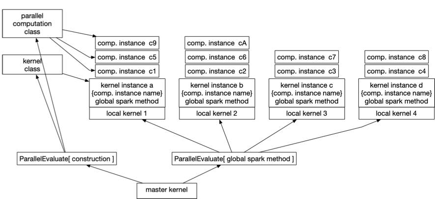
Part 2 is concerned with calculations using multiple instances deployed on each single local kernel, and the method is illustrated in the Mersenne number calculation example.

fig.1 How to deploy and run multiple parallel computing instances on each local kernel

step.1 setup local kernels

LaunchKernels[];
kernelList = ParallelEvaluate[$KernelID];
nk = Length[kernelList];
{nk, kernelList}

step.2 preparing the association list for kernel instances

kernelObject = 
 Table[Association["name" -> Unique[k], 
   "kernel" -> kernelList[[i]]], {i, nk}]

step.3 preparing the association list for parallel computing instances

object = {
   Association["name" -> Unique[c], "range" -> {9000, 9299}, 
    "kernel" -> 1],
   Association["name" -> Unique[c], "range" -> {9300, 9399}, 
    "kernel" -> 2],
   Association["name" -> Unique[c], "range" -> {9400, 9499}, 
    "kernel" -> 3],
   Association["name" -> Unique[c], "range" -> {9500, 9599}, 
    "kernel" -> 4],
   Association["name" -> Unique[c], "range" -> {9600, 9699}, 
    "kernel" -> 1],
   Association["name" -> Unique[c], "range" -> {9700, 9799}, 
    "kernel" -> 2],
   Association["name" -> Unique[c], "range" -> {9800, 9899}, 
    "kernel" -> 3],
   Association["name" -> Unique[c], "range" -> {9900, 10000}, 
    "kernel" -> 4]
   };

step.4 construct a table for the parallel computing instances that will be deployed to each local kernel

prNameTable = 
 Table[Map[#name &, 
   Select[object, #kernel == kernelNumber &]], {kernelNumber, 4}]

step.5 definition of local kernel class

object1 = {
  Association["name" -> Unique[c], "range" -> {9000, 9299}],
  Association["name" -> Unique[c], "range" -> {9300, 9399}]}

kernel[nam_[myKernelNumber_]] := 
 Module[{myID = nam, localInstance = {}},
  getID[] := myID;
  namset[myObject_] := localInstance = myObject;
  para[nam_[{ns_, ne_}]] := Module[{myID = nam, ins = ns, ine = ne},
    nam[getID] := myID;
    nam[getStatus] := {ins, ine};
    go[nam] ^:= Select[Range[ins, ine], PrimeQ[2^# - 1] &]];
  Map[para[#name[#range]], localInstance];
  spark[] := Map[go[#] &, localInstance];
  ]

step.6 construction of kernel instances and deployment to each core

Map[ParallelEvaluate[kernel[#name[#kernel]], #kernel] &, kernelObject]

step.7 definition of parallel computation class

para[nam_[{ns_, ne_}]] := Module[{myID = nam, ins = ns, ine = ne},
   nam[getID] := myID;
   nam[getStatus] := {ins, ine};
   go[nam] ^:= Select[Range[ins, ine], PrimeQ[2^# - 1] &]];

step.8 construction of parallel computation instances and deployment to the kernel instances

Map[ParallelEvaluate[para[#name[#range]], #kernel] &, object]

ParallelEvaluate[object1, 1]

ParallelEvaluate[namset[k$2984[object1]], 1]

strp.9 execute parallel computing

ts = SessionTime[];
ans = ParallelEvaluate[spark[]];
{SessionTime[] - ts, ans}

Results of the computation on my environment is,

{11.947488, {{{}, {9689}}, {{}, {}}, {{}, {}}, {{}, {9941}}}}

The above calculation results show that the calculation results from two parallel calculation instances are returned from each of the four kernels. For example, the beginning of the list included in the calculation returned by the list is {{}, {9689}}. This indicates that the first kernel ran two parallel computation instances, of which the second parallel computation found the Mersenne number. At the same time, you can see that the fourth kernel executed by the second kernel also found another Mersenne number.