In[5]:= sphcmpt[pefunc, nInteger, d_] := Block[{i, vars, psi, vwb, ener, enres, psires, varres, cons1, cons2, sln, wavefunctions}, (* define variables *) vars = Table[psi[r], {r, 0, 1, d}];

  (* add bounds to variables *)
  vwb = {#, -1000, 1000} & /@ vars;

  (* calculate expectation values of energy for a radial function \
using finite differences with spacing d for derivatives *)
  ener = d Sum[-psi[
         r] (2/r ((psi[r + d] - psi[r - d])/(2 d)) + ((
          psi[r + d] - 2*psi[r] + psi[r - d])/d^2)) 4 \[Pi] r^2 + 
      psi[r] pefunc psi[r] 4 \[Pi] r^2, {r, d, 1 - d, d}]; 

  (* allocate variables for results *)
  enres = Table[0, n];
  wavefunctions = Table[0, n];

  (* boundary condition and normalization condition *)
  cons1 = {psi[1] == 0, 
    4  \[Pi] Sum[r^2 psi[r]^2, {r, d, 1, d}] == d^-1};

  (* calculate lowest n energy levels *)
  Do[
   (* orthogonality constraints *)
   cons2 = 
    Table[Sum[
       psi[r]*(psi[r] /. wavefunctions[[j]])*r^2, {r, 0, 1, d}] == 
      0, {j, i - 1}];

   (* use ParametricIPOPTMinimize to solve problem, 
   using 10 random searches, seed 0 *)
   sln = iMin[ener, Join[cons1, cons2], vwb, 10, 0];

   (* save results *)
   enres[[i]] = sln[[1]];
   wavefunctions[[i]] = sln[[2]],
   {i, n}
   ]; {enres, wavefunctions}
  ]

In[6]:= (* perform calculation *)
hatom = sphcmpt[(-100)/r, 5, 10^-3];

During evaluation of In[6]:= {{Solve_Succeeded,10}}

During evaluation of In[6]:= {{Solve_Succeeded,10}}

During evaluation of In[6]:= {{Solve_Succeeded,10}}

During evaluation of In[6]:= {{Solve_Succeeded,10}}

During evaluation of In[6]:= {{Solve_Succeeded,10}}

In[7]:= (* look at energy levels *)
hatom[[1]]

Out[7]= {-2498.44, -624.902, -277.758, -156.015, -89.3199}

In[8]:= (* check that energy levels go as 1/n^2 *)
Table[hatom[[1, i]]*i^2, {i, 5}]

Out[8]= {-2498.44, -2499.61, -2499.83, -2496.25, -2233.}

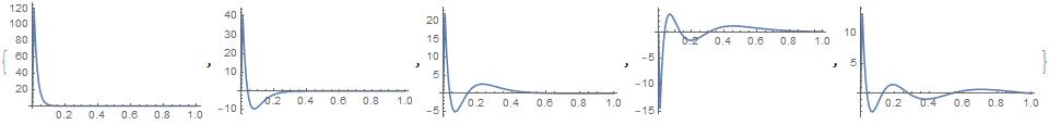
In[9]:= (* Plot wavefunctions *)
Table[ListPlot[Table[{r, psi[r]}, {r, 0, 1, 1/100}] /. hatom[[2, n]], 
  Joined -> True, PlotRange -> All], {n, 5}]

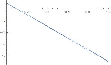
(* Verify that lowest state is exponential in r *)
ListPlot[Table[{r, Log @ psi[r]}, {r, 0, 1, 1/100}] /. hatom[[2, 1]]]