Energy Levels and Wavefunctions in a 2-D Infinite Square Well Potential are Computed By Minimizing the Expectation Values of the Wavefunction Energies.
In[5]:= cmpt[pefunc_ (* potential energy function *),
n_Integer (* number of wavefunctions to compute *),
d_ (* discretization size *),
max_ (* max value of wave function *),
nrands_Integer (* number of random starts *),
seed_Integer (* random seed *)] :=
Block[{pts, npts, vars, psi, vwb, sides, bcons, normcond, ke, pe,
ener, enres, varres, wavefunctions, orthogcons, allcons, sln},
(* points at which wavefunction is calculated *)
pts = Flatten[Table[{x, y}, {x, -1, 1, d}, {y, -1, 1, d}], 1];
(* number of points *)
npts = Length[pts];
(* optimization variables *)
vars = Table[psi[pts[[i]]], {i, npts}];
(* optimization variables with bounds *)
vwb = {#, -max, max} & /@ vars;
(* boundaries of region *)
sides = Select[pts, Or[#[[1]]^2 == 1, #[[2]]^2 == 1] &];
(* boundary conditions *)
bcons = Table[psi[sides[[i]]] == 0, {i, Length[sides]}];
(* normalization condition *)
normcond = vars.vars == npts;
(* total kinetic energy computed using finite differences *)
ke = -npts^-1 (Sum[
psi[{x, y}] ((
psi[{x + d, y}] - 2*psi[{x, y}] + psi[{x - d, y}])/
d^2), {x, -1 + d, 1 - d, d}, {y, -1, 1, d}]
+ Sum[
psi[{x, y}] ((
psi[{x, y + d}] - 2*psi[{x, y}] + psi[{x, y - d}])/
d^2), {y, -1 + d, 1 - d, d}, {x, -1, 1, d}]);
(* total potential energy *)
pe = npts^-1 Sum[
psi[{x, y}]*pefunc*psi[{x, y}], {x, -1, 1, d}, {y, -1, 1, d}];
(* total energy *)
ener = ke + pe;
(* setup results *)
enres = Table[0, n];
varres = Table[0, n];
wavefunctions = Table[0, n];
(* perform calculation *)
Do[
(* wave function is orthogonal to wave functions of lower energy \
states *)
orthogcons = Table[vars.varres[[j]] == 0, {j, i - 1}];
(* all constraints *)
allcons = Join[bcons, {normcond}, orthogcons];
(* perform optimization,
minimizing total energy subject to constraints *)
sln = iMin[ener, allcons, vwb, nrands, seed];
(* save results *)
enres[[i]] = sln[[1]];
wavefunctions[[i]] = sln[[2]];
varres[[i]] = vars /. sln[[2]],
{i, n}
];
(* return results *)
{enres, wavefunctions}
]
In[6]:= AbsoluteTiming[sqrwell = cmpt[0, 9, 1/20, 5, 1, 0];]
During evaluation of In[6]:= {{Solve_Succeeded,1}}
During evaluation of In[6]:= {{Solve_Succeeded,1}}
During evaluation of In[6]:= {{Solve_Succeeded,1}}
During evaluation of In[6]:= {{Solve_Succeeded,1}}
During evaluation of In[6]:= {{Solve_Succeeded,1}}
During evaluation of In[6]:= {{Solve_Succeeded,1}}
During evaluation of In[6]:= {{Solve_Succeeded,1}}
During evaluation of In[6]:= {{Solve_Succeeded,1}}
During evaluation of In[6]:= {{Solve_Succeeded,1}}
Out[6]= {51.5751, Null}
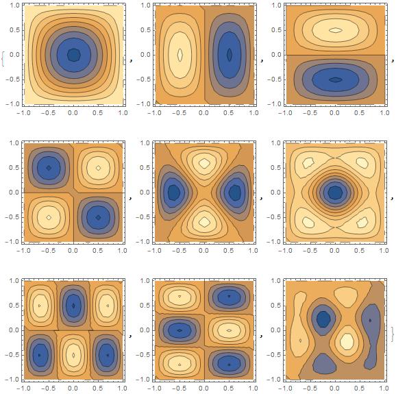
In[7]:= sqrwell[[1]] (* energy levels *)
Out[7]= {4.93227, 12.3155, 12.3155, 19.6987, 24.5702, 24.5702, \
31.9534, 31.9534, 41.6209}
In[8]:= (* theoretical dependence of energy levels on quantum numbers \
*)
theorlevels = Sort @ Flatten[Table[n1^2 + n2^2, {n1, 3}, {n2, 3}]]
Out[8]= {2, 5, 5, 8, 10, 10, 13, 13, 18}
In[9]:= Table[
sqrwell[[1, i]]/theorlevels[[i]], {i,
9}] (* test computed energy levels *)
Out[9]= {2.46613, 2.46309, 2.46309, 2.46233, 2.45702, 2.45702, \
2.45795, 2.45795, 2.31227}
In[10]:= (* plot wavefunctions *)
Table[ListContourPlot[
Flatten[Table[{x, y, psi[{x, y}]}, {x, -1, 1, 1/10}, {y, -1, 1,
1/10}] /. sqrwell[[2, i]], 1], PlotRange -> All], {i, 9}]
 Attachments:


