In[1]:= (* Basis states are Sqrt[2] Sin[n \[Pi] x]*)
    bas[n_][x_] = Sqrt[2] Sin[n \[Pi] x];

In[2]:= 
(* Basis states are normalized *)
FullSimplify[Integrate[bas[n][x]^2, {x, 0, 1}], 
 Assumptions -> n \[Element]  Integers]

Out[2]= 1

In[3]:= 
(* Basis states are 0 at x = 0 and x = 1 *)
Simplify[{bas[n][0], bas[n][1]},  
 Assumptions ->  n \[Element]  Integers]

Out[3]= {0, 0}

In[4]:=  (* Hamiltonian operator is -\[HBar]^2/(2m)d^2/dx^2 + V(x). (\
\[HBar]^2/(2m)) is set equal to 1 and V(x) is set equal to v0 \
(x-1/2)^2 .  
v0 will be large so that the boundary conditions at x = 0 and x = 1 
will be a good approximation to the free simple harmonic oscillator *)


hamop = (v0 (x - 1/2)^2*#) - D[#, {x, 2}] &;

In[5]:= (* Hamiltonian matrix element between states m and n *)
ham[m_, n_] = 
 FullSimplify[Integrate[bas[m][x]*hamop @  bas[n][x], {x, 0, 1}], 
  Element[{m, n}, Integers]]

Out[5]= (4 (1 + (-1)^(m + n)) m n v0)/((m^2 - n^2)^2 \[Pi]^2)

In[6]:= (* Previous result is erroneous when m = n so this case is \
calculated separately *)
ham[n_, n_] = 
 FullSimplify[Integrate[bas[n][x]*hamop @  bas[n][x], {x, 0, 1}], 
  Element[n, Integers]]

Out[6]= n^2 \[Pi]^2 + v0/12 - v0/(2 n^2 \[Pi]^2)

In[7]:= (* Calculate a 100 x 100 Hamiltonian Matrix *)
AbsoluteTiming[
 hamMatrix = Table[N @ ham[m, n], {m, 1, 100}, {n, 1, 100}];]

Out[7]= {0.0598937, Null}

In[8]:= (* Calculate the Eigensytem for the cae when v0 = 10^6  *)
AbsoluteTiming[res = Eigensystem[hamMatrix /. v0 -> 10^6];]

Out[8]= {0.0292793, Null}

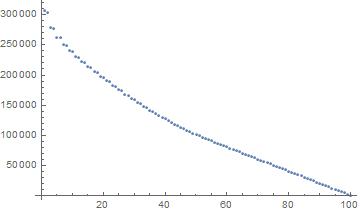
In[9]:=  (* The energy levels are in reverse order *)
ListPlot[res[[1, All]]]

In[10]:=  (* Expected energy levels are (n + 1/2) \[HBar] \[Omega] = \
(n + 1/2) \[HBar] Sqrt[k/m] 
where k is the "spring constant" in the equation and n = 0, 1, 2, etc.
k = 2 v0 since force is gradient of poential, so energy levels = (n + \
1/2) \[HBar] Sqrt[2 v0/m] = (n+1/2) Sqrt[2 v0]  since \[HBar]^2/(2m) \
was set to 1 *)

In[11]:= Simplify[
 Solve[{\[Delta]E == \[HBar] Sqrt[2 v0/m],  (\[HBar]^2)/(2 m) == 
    1}, {\[Delta]E, m}], Assumptions -> \[HBar] > 0]

Out[11]= {{\[Delta]E -> 2 Sqrt[v0], m -> \[HBar]^2/2}}

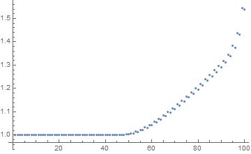
In[12]:= (* The energy levels are correct up to about the 50th energy \
level *)
ListPlot[Table[res[[1, -i]]/(2 10^3 (i - 1/2)), {i, 100}]]

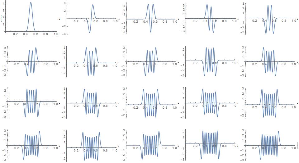
(* Plot the first 20 lowest energy wavefunctions *)
Table[Plot[Sum[res[[2, -i, m]] bas[m][x], {m, 1, 100}], {x, 0, 1}, 
  PlotRange -> All], {i, 20}]