Anderson,

I'm glad I was able to help! My only comment is that your graph is labeled in Milligrams, don't you need to convert to milligrams (or multiply by 1000)? or am I missing something?

Regards,

Neil

Anderson,

The bug has to do with units in the variable of the plot command. A simple workaround is to take the units out of the plot command and put it into your expression:

Plot[UnitConvert[m[Quantity[t, "Seconds"]], "Milligrams"], {t, 0, 10},
  AxesLabel -> {"t(s)", "m(g)"}]

Now you can do the conversion to milligrams in MMA avoiding any problems.

Alternatively you can add the units of seconds in the definition of m[t]:

mm[t_] := 
  Module[{newt = 
     Quantity[t, "Seconds"]}, (c1 newt^(8/10) + c2 newt + c3) /. 
    regData];

and plot with the simple command:

Plot[UnitConvert[mm[t], "Milligrams"], {t, 0, 10}, 
 AxesLabel -> {"t(s)", "m(g)"}]

Regards,

Neil

My approach to this would be to disentangle the graphics from the units and then use a simplified approach to specifying the graphics. I do this with two applications I've written. If you would like a copy of them just write me and I'll give you the link. (UnitsHelper, among other features, has decibel units and provision for specifying reduced unit systems such as gravitational units or atomic units.)

<< UnitsHelper`
<< Presentations`

The first step is to deunitize the the mass expression that has units in it to obtain a numerical expression with implicit units. Define the mass expression:

mass = c1 t^(4/5) + c2 t + c3;

We have to specify that the variables are numeric.

TagSet[#, NumericQ[#], True] & /@ {c1, c2, c3, t}; 

Define the data for the expression. There is one extra definition specifying the units for t.

data = {c1 -> Quantity[5.00, "Grams"/("Seconds")^(8/10)], 
  c2 -> Quantity[-3.00, "Grams"/"Seconds"], 
  c3 -> Quantity[20.00, "Grams"], t -> t Quantity[1, "Seconds"]};

We then use a UnitsHelper routine, ToImpliedUnits, on the mass expression. We supply the data rules and the output unit. We could have used any set of units for these as long as they are consistent. The result is an Association.

(resultAssoc = mass // ToImpliedUnits[data, Quantity[1, "Grams"]]) // 
  Normal // Column

Giving

<|"Expression" -> c3 + c1 t^(4/5) + c2 t, 
 "Data" -> {c1 -> Quantity[5., ("Grams")/("Seconds")^(4/5)], 
   c2 -> Quantity[-3., ("Grams")/("Seconds")], 
   c3 -> Quantity[20., "Grams"], t -> Quantity[t, "Seconds"]}, 
 "Variable Units" -> {t}, "Output Units" -> "Grams", 
 "Implied Expression" -> 20. + 5. t^(4/5) - 3. t|>

Define the numeric expression by extracting the "ImpliedExpression" from the Association. We define the numerical mass expression. This, of course, would look different if there we used different units.

NMass[t_] = resultAssoc["Implied Expression"]

giving

20. + 5. t^(4/5) - 3. t

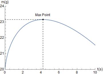
Calculate the time of maximum mass.

tmax = Solve[NMass'[tt] == 0, {tt}][[1, 1, 2]]  

giving

4.21399

Now specify the graphics using a portion of the Presentations application. The idea here is that everything is a Graphics primitive, whereas in Wolfram graphics everything is Graphics. So in the following statement Draw is functionally the same as Plot except that it returns primitives and only uses Options that directly affect the rendering of the curve. It's just drawing one thing after another and specifying everything in one statement that's easy to edit in perfecting a graphic.

Draw2D[
 {Draw[NMass[t], {t, 0, 10}],
  {Dashed, Line[{{0, NMass[tmax]}, {tmax, NMass[tmax]}, {tmax, 0}}]},
  {PointSize[Medium], Point[{tmax, NMass[tmax]}]},
  Text[Style["Max Point", Black, 12], {tmax, NMass[tmax]}, {0, -2}]},
 AspectRatio -> 0.7,
 PlotRange -> {{0, 10}, {20, 24}},
 Axes -> True,
 AxesLabel -> {"t(s)", "m(g)"},
 LabelStyle -> {Black, 12}
 ]

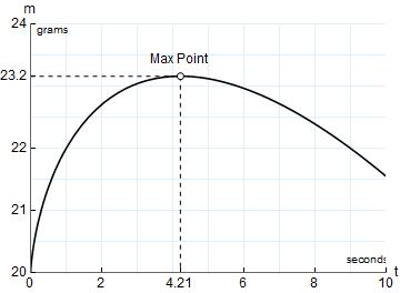
Here is a variation. The Ticks are modified so the coordinates of the max point are shown. A faint LightBlue grid is put in the background. The curve color is changed to Black. A CirclePoint (from Presentations) is used to mark the maximum point. The axis units are marked more explicitly.

xticks = CustomTicks[Identity, 
   databased[{{0, 0}, {2, 2}, {tmax, NumberForm[tmax, {3, 2}]}, {6, 
      6}, {8, 8}, {10, 10}}]];
yticks = CustomTicks[Identity, 
   databased[{{20, 20}, {21, 21}, {22, 22}, {NMass[tmax], 
      NumberForm[NMass[tmax], {3, 1}]}, {24, 24}}]];
Draw2D[
 {Draw[NMass[t], {t, 0, 10}, PlotStyle -> {Black}],
  {Dashed, Line[{{0, NMass[tmax]}, {tmax, NMass[tmax]}, {tmax, 0}}]},
  CirclePoint[{tmax, NMass[tmax]}, 3, Black, White],
  Text[Style["Max Point", Black, 12], {tmax, NMass[tmax]}, {0, -2}],
  Text["grams", {0.2, 23.9}, {-1, 0}],
  Text["seconds", {9.5, 20.2}]
  },
 AspectRatio -> 0.7,
 PlotRange -> {{0, 10}, {20, 24}},
 Axes -> True,
 AxesLabel -> {"t", "m"},
 Ticks -> {xticks, yticks},
 GridLines -> {CustomGridLines[Identity, {0, 10, 1}], 
   CustomGridLines[Identity, {20, 24, 1/2}]},
 Method -> {"GridInFront" -> False},
 LabelStyle -> {Black, 12}
 ]

Nothing funny happens.

... especially the "Plot functions of Quantities with Units?", posted by Eric Hudson in this community.

Obviously this problem still exists (v12.0) and still one good workaround is using ListLinePlot instead. I would do it like so:

regData = {c1 -> Quantity[5.00, "Grams"/("Seconds")^(8/10)], c2 -> Quantity[-3.00, "Grams"/"Seconds"], c3 -> Quantity[20.00, "Grams"]};

m[t_] := Evaluate[(c1 t^(8/10) + c2 t + c3) /. regData];

data = Table[{t, m[t]}, {t, Quantity[0., "Seconds"], Quantity[10., "Seconds"], Quantity[.1, "Seconds"]}];
sol1 = Solve[m'[t] == 0, t] // Flatten;

ti = 0;
tf = QuantityMagnitude[t /. sol1];
mi = 0;
mf = QuantityMagnitude[m[t] /. sol1];

ListLinePlot[data, AxesLabel -> Automatic, 
 Epilog -> {Dashed, Line[{{ti, mf}, {tf, mf}}], Line[{{tf, mi}, {tf, mf}}], PointSize[Medium], Point[{tf, mf}], Text["Max point", {1.3 tf, 1.004 mf}]}]

Instead of defining different graphics and adding them together with Show the command Epilog can be used, but sadly quantities are understood here neither. Just for making the quantities used obvious I changed AxesLabel to Automatic.