Introduction:

In this work, I explore the sequence A023393-OEIS (definition: “maximum number of circles of radius 1 that can be packed in a circle of radius n”, author: David W. Wilson, last approved on September 29, 2013). It is a sequence in which the function does not have a closed form or clear defined equation, and appears at its discretion: "…(terms) are only conjectures supported by extensive calculations". It is considered "hard" in its definition; this means that it is difficult to calculate its terms.

Approach:

I was able, using Wolfram Language and the GeometricScene feature, to create a computational model to calculate the terms of this complicated sequence (all the codes here are in some way related to this command, even the outline drawing).

Here, I detail the model (done in conjunction with RandomInstance) while expose its visualization and discuss its limitations.

Designing the Model:

• Sketch:

First, I made an outline of how the model should behave in terms of boundary.

gm = RandomInstance[
     GeometricScene[{a, b, 
       c}, {EuclideanDistance[a, Point[{0, 0}]] == 9,
       EuclideanDistance[b, Point[{0, 0}]] == 2, 
       EuclideanDistance[c, Point[{0, 0}]] == 2, 
       EuclideanDistance[b, c] == 2,
       GeometricAssertion[{Circle[a, 1], Circle[b, 1], Circle[c, 1], 
         Circle[{0, 0}, 10]}]}]]["Points"][[;; 3]];
Show[{Graphics@Circle[{0, 0}, 10], Graphics@Circle[(a /. gm[[1]]), 1],
   Graphics@Circle[(b /. gm[[2]]), 1], 
  Graphics@Circle[(c /. gm[[3]]), 1], 
  Graphics[{Text[Style["max.distance \[LessEqual] R-r", Blue, 12], 
     Midpoint[Line[{(a /. gm[[1]]), {0, 0}}]]], Red, Dashed, 
    Line[{(a /. gm[[1]]), {0, 0}}]}], 
  Graphics[{Text[Style["min.distance \[GreaterEqual] 2.r", Blue, 12], 
     Midpoint[Line[{(b /. gm[[2]]), (c /. gm[[3]])}]] + 1.5], Red, 
    Dashed, Line[{(b /. gm[[2]]), (c /. gm[[3]])}]}], 
  Graphics[{Red, Dashed, Circle[{0, 0}, 9]}]}]

• Scattering:

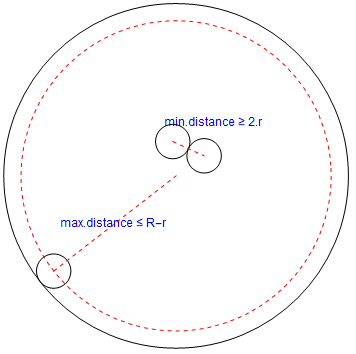
A way to random scatter the points (centers of small circles).

f[n_] := Module[{a, b, c, d}, 
   a = Table[(StringJoin[{"p", i // ToString}] // ToExpression), {i, 
      1, n}]; b = Subsets[a, {2}]; 
   c = Table[
     EuclideanDistance[b[[j, 1]], b[[j, 2]]] >= 2, {j, 1, Length@b}]; 
   d = GeometricAssertion[Table[Point[a[[k]]], {k, 1, Length@a}]]; 
   RandomInstance[GeometricScene[{a, {}}, Evaluate@Join[c, {d}]]]];
f[15]

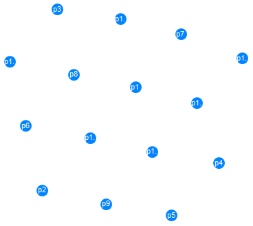
It is easy to find the coordinates of the points (example).

po = %["Points"]

Just to measure dispersion (not necessary for the final result): find the shortest distance between any of the generated points (Min) and the maximum dispersion distance of the points (Max).

n = Length@po; u1 = 
 Table[(StringJoin[{"p", i // ToString}] // ToExpression), {i, 1, 
   n}]; u2 = 
 Subsets[u1 /. po, {2}]; Thread[{{"Min", "Max"}, 
  Map[#@Map[EuclideanDistance[u2[[#, 1]], u2[[#, 2]]] &, 
      Range@Length@u2] &, {Min, Max}]}]

• Packing in a circle:

Now, limiting the scatter within a larger circle and defining a raw view.

g[n_, v_] := 
  Module[{a, b, c, d, cx, dx}, 
   a = Table[(StringJoin[{"p", i // ToString}] // ToExpression), {i, 
      1, n}]; b = Subsets[a, {2}]; 
   cx = Table[
     EuclideanDistance[b[[j, 1]], b[[j, 2]]] >= 2, {j, 1, Length@b}]; 
   dx = Table[
     EuclideanDistance[a[[s]], Point[{0, 0}]] <= v - 1, {s, 1, 
      Length@a}]; c = Join[cx, dx]; 
   d = GeometricAssertion[
     Join[Table[
       Circle[a[[k]], 1], {k, 1, Length@a}], {Circle[{0, 0}, v]}]]; 
   RandomInstance[GeometricScene[{a, {}}, Evaluate@Join[c, {d}]]]];
g[30, 10]

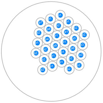
• Maximizing the number of circles:

With the preview of the model ready, I was able to create a code that estimates the maximum number of small circles that can be packaged. Limited to an operational time defined using TimeConstrained (this code is relatively slow because it searches for an answer; there is a loop that goes up and a loop that goes down in order to scan for a result). The usefulness of this code is to give an estimate in advance of the number of circles that should be used in the final model.

MaxCircles[ratio_, time_: 5] := 
  Module[{h, y}, 
   num[n_, v_, t_] := 
    Module[{a, b, cx, dx, c, d}, 
     a = Table[(StringJoin[{"p", i // ToString}] // ToExpression), {i,
         1, n}]; b = Subsets[a, {2}]; 
     cx = Table[
       EuclideanDistance[b[[j, 1]], b[[j, 2]]] >= 2, {j, 1, 
        Length@b}]; 
     dx = Table[
       EuclideanDistance[a[[s]], Point[{0, 0}]] <= v - 1, {s, 1, 
        Length@a}]; c = Join[cx, dx]; 
     d = GeometricAssertion[
       Join[Table[
         Circle[a[[k]], 1], {k, 1, Length@a}], {Circle[{0, 0}, v]}]]; 
     TimeConstrained[
      RandomInstance[GeometricScene[{a, {}}, Evaluate@Join[c, {d}]]], 
      t]]; If[y = 1; h = 1; 
    While[True, If[num[h, ratio, time] == $Aborted, Break[]]; h++]; 
    num[h - 1, ratio, time] == $Aborted, 
    While[True, If[num[h - y, ratio, time] != $Aborted, Break[]]; 
     y++]]; {Style[StringJoin["Circles: ", (h - y) // ToString], 
     Large], num[h - y, ratio, time]}];

MaxCircles[5]

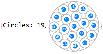
Final Model:

With everything ready, it was possible to generate the final model below (in the code “n” is the number of small circles, “v” is the radius of the large circle, “ra” is the radius of the small circle that automatically has a value of 1 and “t” is the maximum time of operation, which by default is 300 seconds, but also can be changed):

SceneFillCircles[n_, v_, ra_: 1, t_: 300] := 
  TimeConstrained[
   Module[{a, b, cx, dx, c, d, o1}, 
    a = Table[(StringJoin[{"p", i // ToString}] // ToExpression), {i, 
       1, n}]; b = Subsets[a, {2}]; 
    cx = Table[
      EuclideanDistance[b[[j, 1]], b[[j, 2]]] >= 2*ra, {j, 1, 
       Length@b}]; 
    dx = Table[
      EuclideanDistance[a[[s]], Point[{0, 0}]] <= v - 1*ra, {s, 1, 
       Length@a}]; c = Join[cx, dx]; 
    d = GeometricAssertion[
      Join[Table[
        Point[a[[k]]], {k, 1, Length@a}], {Circle[{0, 0}, v]}]]; 
    o1 = (a /. 
        RandomInstance[
          GeometricScene[{a, {}}, Evaluate@Join[c, {d}]]][
         "Points"])[[;; Length@a]]; 
    Do[Print[{Show@
         Join[{Graphics[{Circle[{0, 0}, v]}], 
           Flatten@
            Table[Graphics[{Hue[RandomReal[]], 
               EdgeForm[Directive[Black]], Disk[o1[[e]], 1*ra]}], {e, 
              1, Length@a}], 
           Graphics@
            Table[Text[Style[e, Black, Large], o1[[e]]], {e, 1, 
              Length@a}]}], o1}[[q]]], {q, 1, 2}]], t, 
   Style["time out", Bold, Red]];

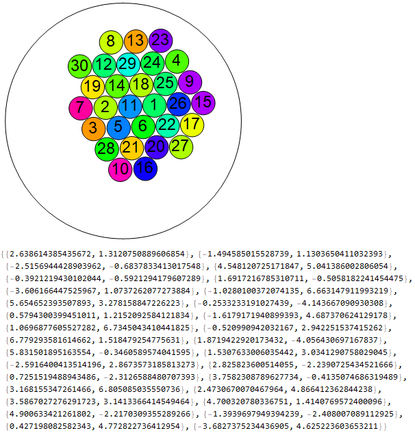
Example of use with partial filling. Note that the result is also available as coordinates of the center of the circles, for example, to generate interactivity later with Manipulate[], Dynamic[], Animate[], etc..

SceneFillCircles[30, 10]

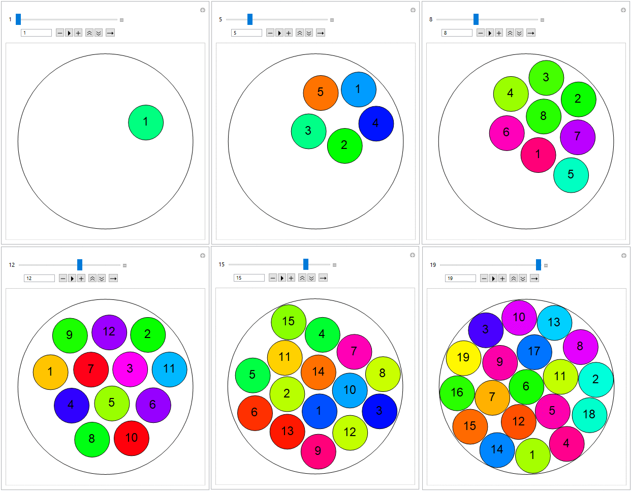
With the help of Manipulate[] and the data obtained from each filling step, it is possible to interactively visualize the behavior of RandomInstance[] with GeometricScene[] in the circle packing. The “data1” line must be filled in with the coordinates of each step (I did not put it here because the code would be unnecessarily large, but it is easy to acquire from the results).

data1 = {"{data n1}, {data n2}, {data n3}, ..."};

v = 5; nu = 19;
Manipulate[
 nn = Table[{EdgeForm[Directive[Black]], Hue[RandomReal[]], 
    Map[Disk[#, 1] &, data1[[n]]][[p]], 
    Text[Style[p, Large, Black], data1[[n]][[p]]]}, {p, 
    Length@data1[[n]]}]; 
 mm = Table[Graphics[nn[[l]]], {l, 1, Length@nn}]; 
 Show@Evaluate@Join[mm, {Graphics[{Black, Circle[{0, 0}, v]}]}], {{n, 
   1, Dynamic[n]}, 1, nu, 1}]

Below is the interactive visualization of the first terms (v=2,v=3,..,v=8), referring to the radius of the larger circle.

data2 = {"{data n1}, {data n2}, {data n3}, ..."};

ini = 2; end = 8;
Manipulate[
 nn = Table[{EdgeForm[Directive[Black]], Hue[RandomReal[]], 
    Map[Disk[#, 1] &, data2[[n - 1]]][[p]], 
    Text[Style[p, Large, Black], data2[[n - 1]][[p]]]}, {p, 
    Length@data2[[n - 1]]}]; 
 mm = Table[Graphics[nn[[l]]], {l, 1, Length@nn}]; 
 Show@Join[mm, {Graphics[{Black, Circle[{0, 0}, n]}]}], {{n, 2, 
   Dynamic[Length@data2[[n - 1]]]}, ini, end, 1}]

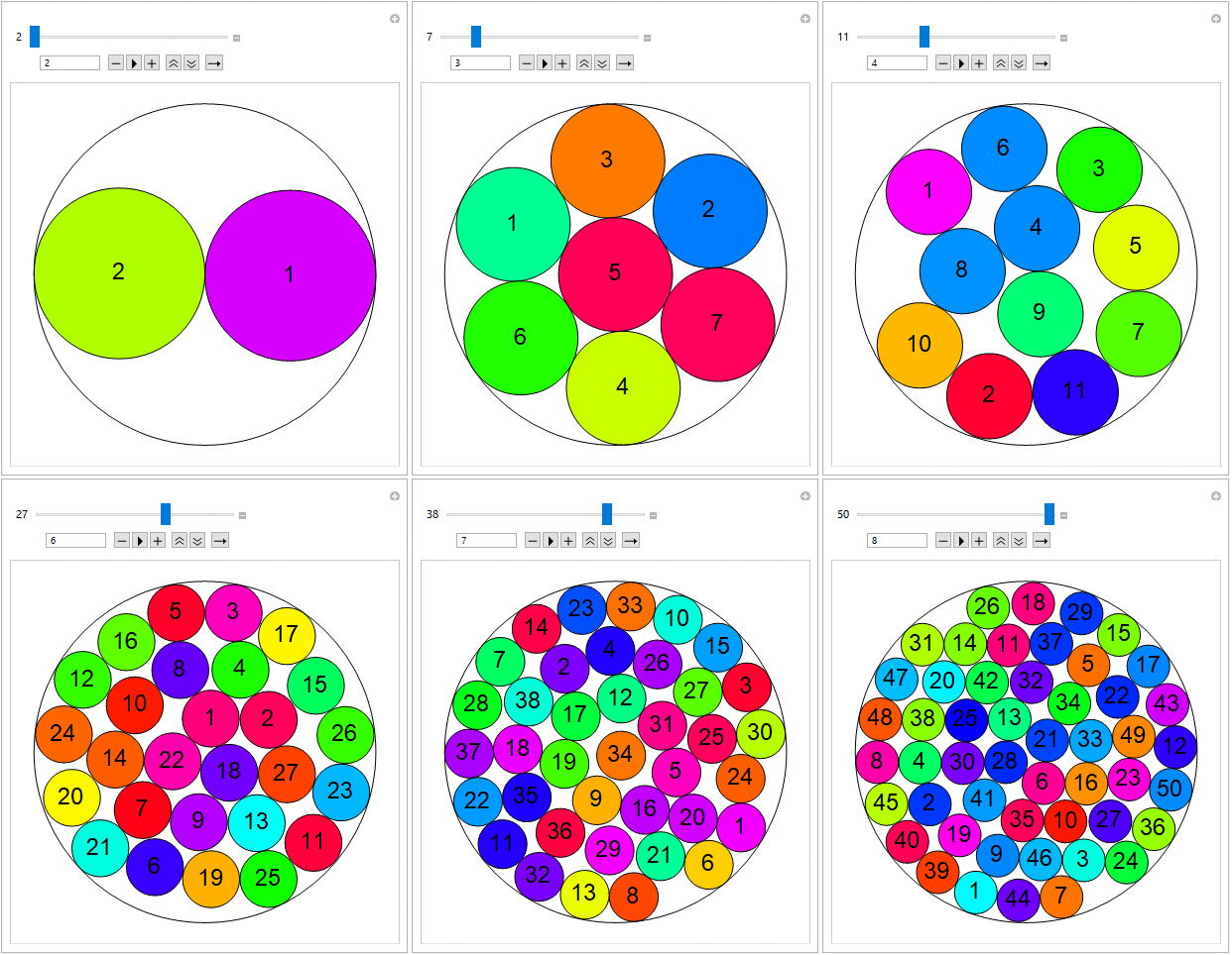
For radii of the greater circle equal to: {v: 2,3,4,5,6,7,8}, the examples below are according with the sequence A023393 OEIS (..successfully confirmed), giving the maximum number of small circles equal to: {n: 2,7,11,19,27,38,50}.

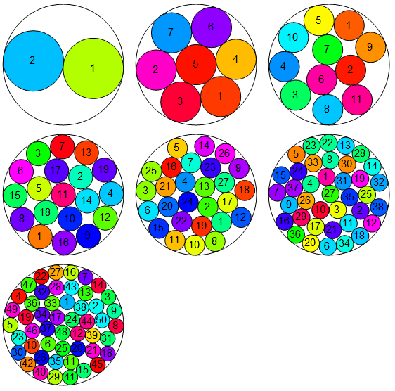
For v>8, there are some difficulties and inaccuracies in the model, as explained in the next section: limitations of the model.

Model Limitations:

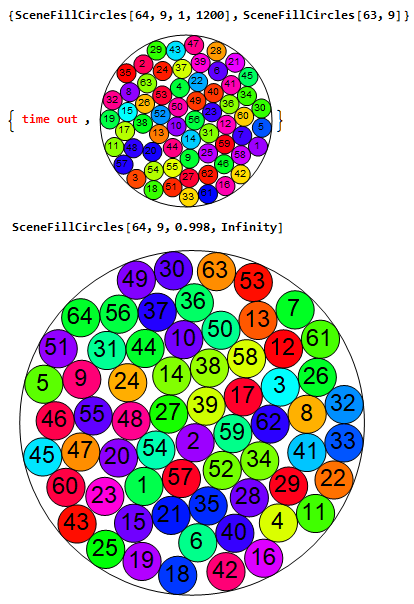
The model created with GeometricScene[] (at least the way I did it) cannot find the number of packaged circles equal to 64 for v=9 (as you would expect through the OEIS sequence). As seen below, even if the available processing time is increased, a result is not found, only a result for 63 circles.

A forced result was found with 64 circles when the radius of the smaller circles was 0.998 instead of 1 (or 0.2% less), but this takes away the accuracy of the model.

Final Notes:

The model presented here has successfully confirmed the first terms (up to a(8)=50) of A023393 OEIS. In addition, it presented the visualizations and data in a computable way.

It would be very interesting to associate this feature with machine learning or neural network to further improve the results and extend this feature (GeometricScene[]) to 3D models (which I believe is not yet possible(?!)).

Despite having some limitations, the GeometricScene[] feature proved to be very useful for creating models in geometric computation. Wolfram Language and Mathematica have enormous potential to explore points that are still not well understood in mathematics.

• Link:

https://oeis.org/A023393

Thanks.