Introduction
This Mathematica code determines the component values for a low-pass active filter implemented using the Sallen-Key architecture. The filter will be a second order Chebyshev filter of type 1. This filter offers a steep cut off at the expense of some passband ripple. It is the location of the poles that define the filter.
The design method is as follows: 1) Derive expressions for the poles of the active filter circuit in terms of the component values; 2) Determine the pole numerical values using Mathematica's Chebyshev1FilterModel; 3) Set the expressions for the pole values equal to the required numerical values and solve for the component values.
Higher order filters can be designed by cascading stages. For example, a 4th order filter can be built by cascading two stages of the same architecture. In this case, the pole values can be determined by using a 4th order Chebyshev1FilterModel. The values are not duplicated: there will be two complex conjugate pairs, one pair for each stage.
SetDirectory[NotebookDirectory[]]; (* for convenience *)
The Sallen-Key architecture
The circuit was drawn with LTSpice, which is a free download. ( https://www.analog.com/en/design-center/design-tools-and-calculators/ltspice-simulator.html# ) It employs an MC33284 op amp as the active component. For work in Mathematica, an ideal op amp will be assumed. Proper selection of the actual op amp makes this a reasonable approximation. 
Circuit design using Mathematica
Some shortcuts
These convenient shortcuts make the circuit equations easier to write and understand.
(* circuit impedances in the s-domain *)
(* inductive impedance *)
xl[l_] := s l;

(* capacitive impedance *)
xc[c_] := 1/(s c);

(* impedance of parallel circuit elements *)
par[z1_, z2_] := (z1 z2)/(z1 + z2);

(* prefixes for numerical quantatives *)
k = 1000.; M = 1.*^6; u = 1.*^-6; p = 1.*^-12;
Transfer function of the Sallen-Key circuit
In this section, we determine the symbolic transfer function Vout/Vin in the s-domain of the above circuit by solving the nodal current equations. We then extract the poles of the transfer function.
(* Node current equations *)
eq1 = (vin - vn)/r1 + (vp - vn)/r2 + (vout - vn)/xc[c2] == 0;
eq2 = (vn - vp)/r2 + (0 - vp)/xc[c1] == 0;

(* Feedback *)
eq3 = vm == vout;

(* op amp transfer function *)
eq4 = (vp - vm) tfOpAmp == vout;

(* r3 balances voltage due to input currents *)
(* it does not effect the transfer function *)
eq5 = r3 == r1 + r2;

(* solve for vout in terms of vin *)
temp = vout /. Solve[{eq1, eq2, eq3, eq4}, vout, {vn, vp, vm}][[1]];

(* transfer function for ideal op amp *)
(* the ideal op amp has infinite gain and no poles or zeros *)
tf = Limit[temp, tfOpAmp -> Infinity]/vin // Simplify;

(* the poles in terms of symbolic component values *)
symbolicPoles =
  TransferFunctionPoles[TransferFunctionModel[tf, s]] // Flatten;
Ideal Chebyshev filter with Fc = 50KHz
In this section, we model a 2nd order 50 KHz Chebyshev low-pass filter using Chebyshev1FilterModel and extract the numerical values of its poles. The filter is a Chebyshev filter of type 1, which exhibits passband ripple. It is the location of the pole pair that determines its type.
fc = 50 k;

cheby50k = Chebyshev1FilterModel[{"LowPass", 2, 2 Pi fc}, s];

poles = TransferFunctionPoles[cheby50k] // Flatten

(* {-101095.54884103949`-244066.24510758917` \
\[ImaginaryI],-101095.54884103949`+244066.24510758917` \[ImaginaryI]} \
*)
Solve for component values
In this section, we set the symbolic expression for the circuit poles to the numerical values of the Chebyshev filter. We set bounds on circuit components and use FindInstance. Note that there are two poles which are complex conjugates, so we only need to use one of them to determine component values.
(* equate the symbolic pole value to the real values determined by \
Mathematica *)
sp1 = symbolicPoles[[1]] == poles[[1]];

(* and find a solution with reasonable component values *)
values = FindInstance[
   sp1 && r1 > 50 k && r2 > 50 k && c1 > 0 && c2 > 0, {r1, r2, c1,
    c2}][[1]]

(* {r1\[Rule]50029.`,r2\[Rule]50040.`,c1\[Rule]2.8951943502775034`*^-\
11,c2\[Rule]1.9769623871729508`*^-10} *)

(* choose close standard values for components *)
standardValues = {r1 -> 50 k, r2 -> 50 k, c1 -> 30 p, c2 -> 200 p};
Check the transfer function with the standard values
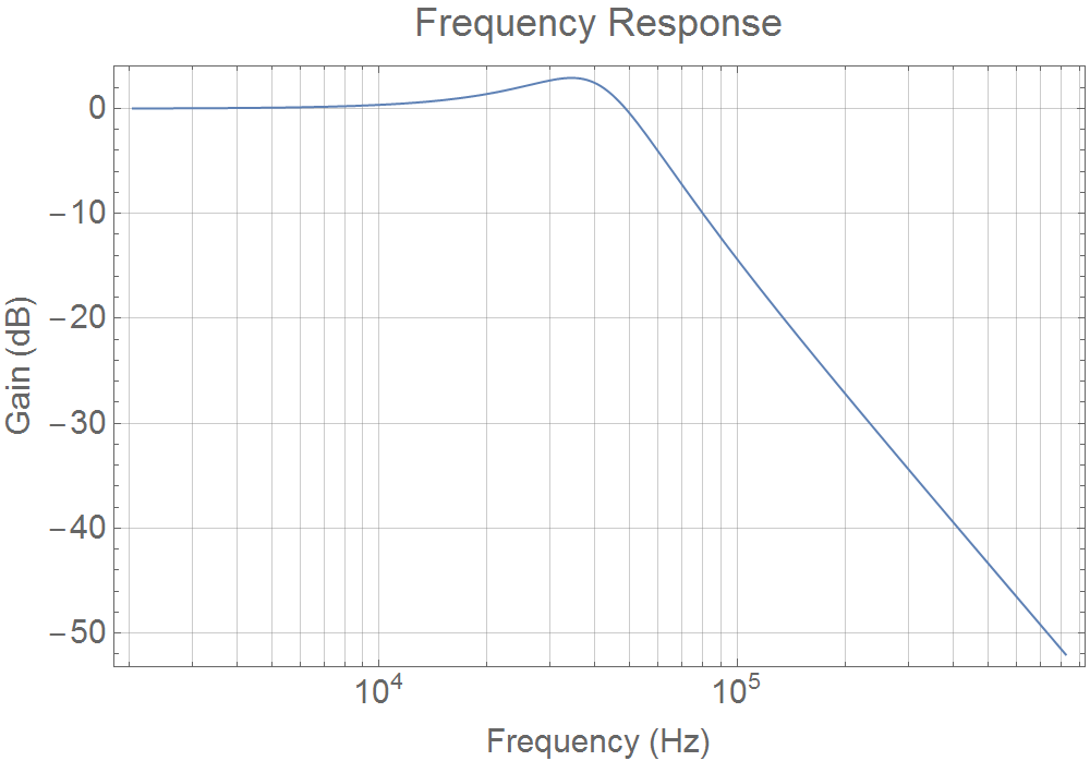
Frequency response
tfm2 = TransferFunctionModel[tf /. standardValues, s];

plot[1] =
 BodePlot[tfm2[2 Pi s], GridLines -> Automatic, FeedbackType -> None,
  ImageSize -> 600, PlotLayout -> "Magnitude",
  PlotLabel -> "Frequency Response",
  FrameLabel -> {"Frequency (Hz)", "Gain (dB)"}, LabelStyle -> 18]
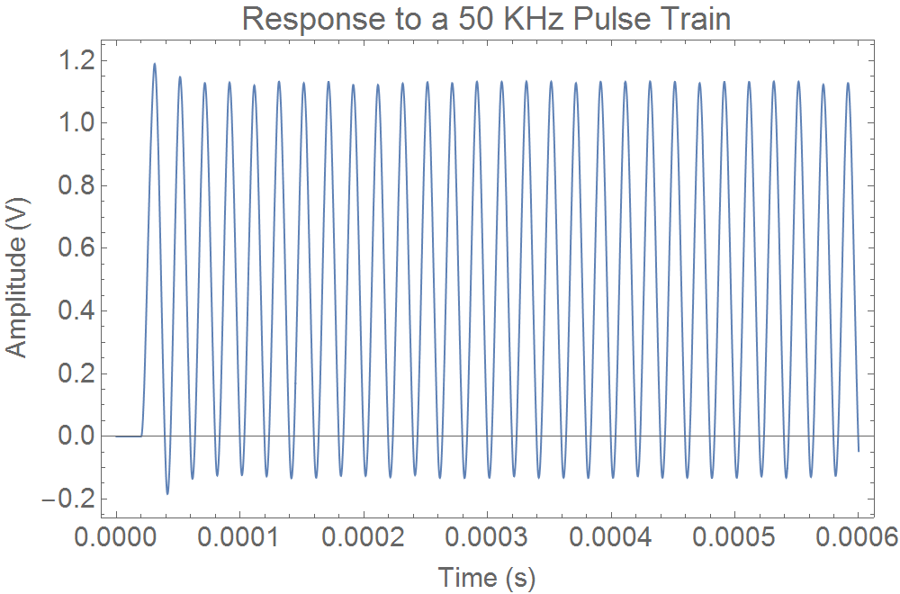
Dynamic response to a 50 KHz pulse train
stimulus = (UnitStep[t - 1/(50 k)]) (SquareWave[50 k t] + 1)/2;

out = OutputResponse[tfm2, stimulus, {t, 0, 60/50000}];

plot[2] = Plot[out, {t, 0, .0006}, ImageSize -> 600, Frame -> True,
  PlotLabel -> "Response to a 50 KHz Pulse Train",
  FrameLabel -> {"Time (s)", "Amplitude (V)"}, LabelStyle -> 18]
(* export the plots *)

export[n_] :=
 Export[ToString@
   StringForm["Sallen-Key Low Pass Filter 1_1 plot-``.png", n],
  plot[n]]

export /@ {1, 2};
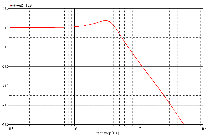
A comparison to a SPICE simulation
The circuit design was simulated using AIMSpice version 2018.100. AIMSpice is also a free download. ( http://www.aimspice.com/ ) It could have been simulated in LTSpice, but I had a device model for the MC33284 op amp available for AIMSpice. We see below that the performance as simulated in SPICE is very similar to that determined in Mathematica. The minor differences are probably caused by the standard component values differing from the ideal, as well as by the fact that in Mathematica we used and ideal op amp (infinite input impedance, zero output impedance, and infinite gain) while AIMSpice used a circuit model for the op amp.
AIMSpice Bode plot
Import["C:\\Users\\David\\Documents\\Electronics\\Active \
filters\\AimSpice Bode.PNG"]
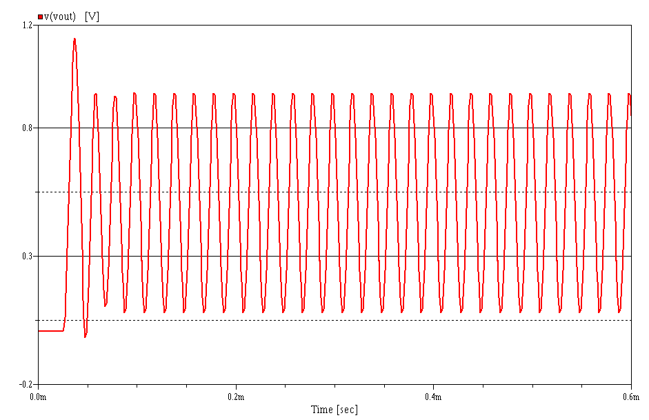
AIMSpice pulse train
Import["C:\\Users\\David\\Documents\\Electronics\\Active \
filters\\AimSpice Pulse.PNG"]
 Attachments:


