Message Boards Message Boards

1
|
7620 Views
|
14 Replies
|
5 Total Likes
View groups...
Share
Share this post:

RegionDifference produces unusable ouput

Posted 4 years ago

I want to create a simple LED optic. I have defined the outer body of the optic and I have defined the 'pin', which is inserted into the main body. These 3D regions are both defined as Implicit Regions. I use RegionDifference to combine them, but the result is corrupted.

Shown below, on the left, is the main body Implicit region. On the right is the region after the RegionDifference has been applied. The inserted pin is not shown in this view. The difference operation has altered the main body and it seems to be 'meshed' at very low resolution.

How can I apply a RegionDifference operation that leads to a non-corrupted output form? The notebook code has been attached.

enter image description here

POSTED BY: Antony Case
14 Replies
Posted 4 years ago

Hi GianLuca,

I cannot help with either of these problems. I am still too new to Mathematica.

Regards

Antony

POSTED BY: Antony Case

Look at this:

Region@ImplicitRegion[
  x^2 + y^2 <= (31981/10000 + z (9/10 + (-(9/250) + z/1000) z))^2 && 
   1/10000 <= z <= 181/20 && 
   Not[x^2 + y^2 <= (31/10 - (35 z)/976)^2 && 
     1/10000 <= z <= 122/25], {x, y, z}]

One of the edges is perfectly drawn on screen. Why not the other?

Also, Mathematica cannot discretize this very, very simple semialgebraic region, that arises from a cylindrical decomposition of our original object:

DiscretizeRegion[
 ImplicitRegion[(13689/1600 < x^2 + y^2 < 36616936723249/
     3810304000000 && 
    15128/175 - 976/35 Sqrt[x^2 + y^2] <= z < 181/20), {x, y, z}], 
 Method -> "Semialgebraic"]
POSTED BY: Gianluca Gorni
Posted 4 years ago

Hi Tim,

What you have posted is amazing. The OpenCascade Link will work for me because I am using Mathematica 12.1. However, I am not really in a position to dive in with OpenCascade yet because I have to get to grips with the core Mathematica. In particular, I must get to grips with NDSolve and investigate the heat performance of this lens.

I have been reading the documentation for OpenCascade and it looks like it is able to Import Step files - something Mathematica can't do. This is interesting. I may be able to get the .Step files for the optics I am interested in - including the one I have recreated in this post. This is something I am going to look into.

Thank you for your help.

Antony

POSTED BY: Antony Case

You can read in step files, but you will need to make sure the extension is in lower case (i.e., "*.step"). I threw together a step file in SolidWorks and read in easily provided I changed the extension from STEP to step.

Needs["OpenCascadeLink`"]
Needs["NDSolve`FEM`"]
shape2 = OpenCascadeShapeImport["E:\\WolframCommunity\\lens.step"];
bmesh2 = OpenCascadeShapeSurfaceMeshToBoundaryMesh[shape2]
groups = bmesh2["BoundaryElementMarkerUnion"];
temp = Most[Range[0, 1, 1/(Length[groups])]];
colors = ColorData["BrightBands"][#] & /@ temp
bmesh2["Wireframe"["MeshElementStyle" -> FaceForm /@ colors]]

step file process

POSTED BY: Tim Laska
Posted 4 years ago

Hi Tim,

This is extremely useful. Maybe, more like a game-changer. I got it working myself about an hour ago. Next week, I will hook it all up with NDSolve properly.

Thank you for telling me OpenCascadeLink. It really will help.

Antony

POSTED BY: Antony Case
Posted 4 years ago

Hi Henrik,

As you may have guessed, I am new to Mathematica and I have been using my lockdown over Easter to dive in. Thank you for your help.You certainly have cleaned everything up.The code I posted had gone through so many edits and tweaks, as I tried more and more to get things to get it to work, that all variable names had become meaningless.

Antony

POSTED BY: Antony Case

If you have version 12.1, then you can use the OpenCascade Link to give access to the open source CAD program. Like most CAD packages, it can do a good job with boolean operations.

I am by no means an expert, but I was able to throw this workflow together based on the tutorial.

(* Load Required Packages *)
Needs["OpenCascadeLink`"]
Needs["NDSolve`FEM`"]
(* parameters *)
z0 = 3.1981; z1 = 0.9; z2 = -0.036; z3 = 0.001;
lowz =  0.0001;
highz = 9.05;
mainR = (z0 + z*(z1 + z*(z2 + z3*z))) /. z -> highz;
highPinz = 4.88;
(* create curve for LED *)
pp = ParametricPlot[{(z0 + z*(z1 + z*(z2 + z3*z))), z}, {z, lowz, 
   highz}, AspectRatio -> Automatic, PlotRange -> {{0, All}, All}, 
  MaxRecursion -> 1, PlotPoints -> 20]
(* Extract points from plot *)
coordinates = First[Cases[Normal[pp], Line[l_] :> l, \[Infinity]]];
(* Convert coordinates to 3D *)
pts = ArrayPad[coordinates, {{0, 0}, {0, 1}}];
pts[[All, {1, 2, 3}]] = pts[[All, {1, 3, 2}]];
(* Create surface of revolution in OpenCascade *)
ll = Line[pts];
wire = OpenCascadeShape[ll];
axis = {{0, 0, 0}, {0, 0, 1}};
sweep = OpenCascadeShapeRotationalSweep[wire, axis];
bmesh = OpenCascadeShapeSurfaceMeshToBoundaryMesh[sweep];
Show[Graphics3D[{{Red, Thickness[0.02], ll}, {Blue, Thick, 
    Arrow[10 axis]}}], bmesh["Wireframe"], Boxed -> False]
(* Cap ends of swept shell *)
crd = bmesh["Coordinates"];
lowcap = Polygon@Select[crd, (#[[3]] == lowz) &];
highcap = Polygon@Select[crd, (#[[3]] == highz) &];
p1 = OpenCascadeShape[lowcap];
p2 = OpenCascadeShape[highcap];
shape = OpenCascadeShapeSewing[{sweep, p1, p2}];
(* Create main body *)
cylshape = 
  OpenCascadeShape[
   c1 = Cylinder[{{0, 0, lowz}, {0, 0, highPinz}}, mainR]];
(* Difference LED from main in OpenCascade *)
diff = OpenCascadeShapeDifference[cylshape, shape];
(* Visualize *)
bmeshshape = OpenCascadeShapeSurfaceMeshToBoundaryMesh[shape];
bmeshcyl = OpenCascadeShapeSurfaceMeshToBoundaryMesh[cylshape];
bmeshdiff = OpenCascadeShapeSurfaceMeshToBoundaryMesh[diff];
groups = bmeshdiff["BoundaryElementMarkerUnion"];
temp = Most[Range[0, 1, 1/(Length[groups])]];
colors = ColorData["BrightBands"][#] & /@ temp;
Show[bmeshshape["Wireframe"], bmeshcyl["Wireframe"]]
bmeshdiff["Wireframe"["MeshElementStyle" -> FaceForm /@ colors]]

open cascade output

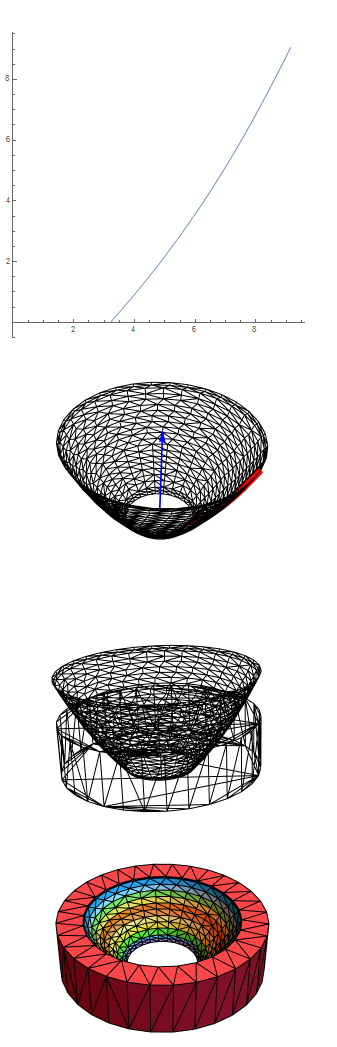
It appears that OpenCascade does a good job maintaining sharp edges.

POSTED BY: Tim Laska

My guess here is that discretization (using DiscretizeRegion[]) is leading to the wrong track. Region is an abstract concept, and if you write (-> your notebook):

Clear["Global`*"];
z0 = 3.1981; z1 = 0.9; z2 = -0.036; z3 = 0.001;
lowz =  0.0001;
highz = 9.05;
highPinz = 4.88;
mainBody = ImplicitRegion[x^2 + y^2 <= (z0 + z*(z1 + z*(z2 + z3*z)))^2 && lowz <= z <= highz, {x, y, z}];
pin =  ImplicitRegion[x^2 + y^2 <= (3.1 - 0.175*z/highPinz)^2 && lowz <= z <= highPinz, {x, y, z}];
df = RegionDifference[mainBody, pin];

then the regions mainBody, pin and df have a clear and clean definition. In fact, we have

enter image description here

I do not know if it makes much sense to write/evaluate Region[df], because df is already a (kind of) region. For displaying regions there are functions like RegionPlot and RegionPlot3D, and here we see that the above issue simply arises due to unsufficient sampling of the regions when plotted:

enter image description here

POSTED BY: Henrik Schachner

If you discretize, your system will not work against the analytical description of the lens, but rather against a bunch of hyper polygons (in 3D), and any computation you do, will have to consider them all, unless you do some programming yourself. This is why I recommended to postpone discretization (if at all) as much as possible.

Good luck with your project

yehuda

Posted 4 years ago

Hi Yehuda,

The command

DiscretizeRegion[df, MaxCellMeasure -> 0.005]

works really well. Thank you, so much. I was really stuck.

My intention is to investigate the thermal performance of the lens with different LEDs. The prospect is that I will need to make the lens just once and once I have it, I can loop over many thermal simulations. The speed of execution for generating the lens is only expected to be a minor issue.

Again thank you.

Antony

POSTED BY: Antony Case

I have been using DiscretizeRegion since the prerelease of version 10, so, various computers (all MACs). After the formal version 10 was released I encountered no problems (was an old 2011 MBP) At the moment I'm using 2017 MBP (16GB RAM, with an internal discrete Radeon 560 GPU with 4GB VRAM), Catalina (10.15.4) and Mathematica 12.1. I wonder if this is system related? yehuda

@Gianluca - MaxCellMeasure -> 0.01 is not small enough. 0.005 provides much better results. I didn't encounter crashes for years using regions. What system do you use (I use Mac Pro and MacBook Pro by Apple).

@Anthony - you could think of several options to tackle this issue. First, the graphical representation on the screen has nothing to do with the real accuracy achieved by Region, since graphical representation is ALWAYS discretized. You could achieve a better behavior from the default Region by replacing all the approximate numbers with accurate ones, i.e., change all floating point numbers to rationals. This will improve the resolution at the wider part. Second, if the thickness is of no importance and speed is an issue, you could use (for both exact and approximate versions...)

BoundaryDiscretizeRegion[df, MaxCellMeasure -> 0.005]

which is a little bit more memory efficient than

DiscretizeRegion[df, MaxCellMeasure -> 0.005]

In your case, I would use discretization as late as possible in my computations to speed it up. HTH yehuda

I tried again now, with version 12.0 on MacBook Pro, Mojave 10.14.6. Crash again with DiscretizeRegion[mainBody].

POSTED BY: Gianluca Gorni

Region computation is very unreliable in Mathematica, and it has been for several years. The kernel has just quit on me with DiscretizeRegion[mainBody]. I have found improvements only by setting a low MaxCellMeasure: DiscretizeRegion[df, MaxCellMeasure -> .01]

POSTED BY: Gianluca Gorni
Reply to this discussion
Community posts can be styled and formatted using the Markdown syntax.
Reply Preview
Attachments
Remove
or Discard

Group Abstract Group Abstract