This project objective is to make analyses for Tokyo Metropolitan Highway known as "Syuto-Ko" that is very complex and narrow, with steep curves. "Syuto-Ko" is the highway network of Tokyo but also the hub of Japan highway network. Because Tokyo area is the collection center having about four hundreds years economical activity history, "Syuto-Ko" had to accept the complexity from the beggining of construction, but having the attractive feature.
For the loop finding and other analysis, Mathematica Graph functions are useful, however, we must prepare a graph expressing the highway root, junction, enterance, exit, and the parking-area. For this purpose, we can use a tool "Graph Editor" which can construct, edit, and convert to a graph from the map of nodes, paths, and labels. For example, over the number of 100 nodes of the map construction is not easy apparently. A graph construction of "Syuto-Ko", even if the parts of the network, may be difficult without the support of the tool.
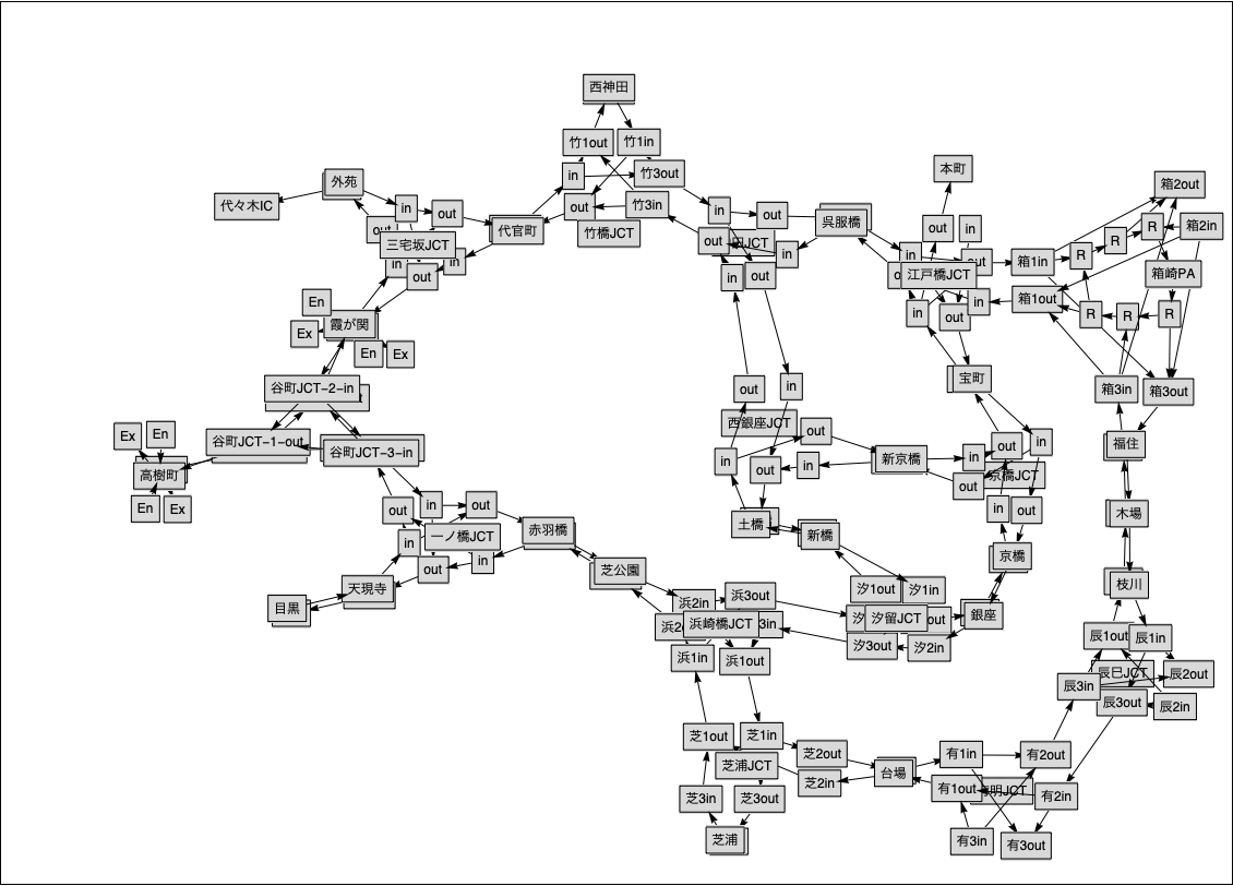
Following figure is a part of Shuto-ko highway drawn by the "Graph Editor," constructed by step by steps. To keep the left, constructed highway map has the inter-change with doubled directions, and the junction point (JCT) has complex in-out directions. All the map are composed of labeled rectangles and the arrows.

Fig.1 Snap shot of working area of GraphEditor
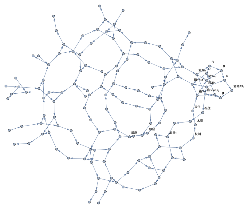
Then, we can convert the map to a graph for the graph functions as following image. Data of Graph function is saved as a file from the GraphEditor command. Converter program source is as follows.
g = Get["graph"][[1 ;; 3]];     (*  read the file *)

f[t_] := Map[Rule[t[[1]], #] &, t[[2]]];     (* define rule function *)

gl1 = Flatten@
   Map[f, Transpose[{Flatten[g[[1]]],
      g[[2]]}]];     (*  construct vertex list of graph  *)

gl1 = gl1 /.
   Rule[x_, y_] /; x == y -> Nothing;     (*  remove self loop *)

gl2 = Map[Rule[#[[1, 1]], #[[2]]] &,
   Transpose[{g[[1]],
     g[[3]]}]];(*  construct label list of graph  *)
gg =
 Graph[gl1, VertexLabels -> gl2, ImagePadding -> 50,
  GraphLayout -> "SpringEmbedding"]
Unfortunately, the number of vertex labels may be limited, you may chose the labels, and can get a graph converted from the GraphEditor file.
gg = Graph[{$138 -> $24, $138 -> $104, $140 -> $146, $140 -> $144, \
$141 -> $110, $142 -> $141, $142 -> $146, $144 -> $145, $145 -> $91, \
$146 -> $28, $147 -> $144, $147 -> $141, $148 -> $147, $149 -> $92, \
$150 -> $156, $156 -> $12, $156 -> $19, $157 -> $102, $160 -> $149, \
$161 -> $164, $161 -> $163, $162 -> $160, $162 -> $164, $163 -> $93, \
$164 -> $150, $166 -> $160, $166 -> $163, $167 -> $148, $169 -> $174, \
$169 -> $171, $170 -> $167, $171 -> $54, $172 -> $170, $172 -> $174, \
$173 -> $171, $173 -> $170, $174 -> $14, $14 -> $16, $14 -> $18, $15 \
-> $178, $16 -> $20, $17 -> $178, $18 -> $134, $33 -> $42, $33 -> \
$44, $34 -> $60, $35 -> $32, $36 -> $42, $41 -> $44, $41 -> $35, $41 \
-> $34, $42 -> $50, $43 -> $42, $43 -> $34, $44 -> $38, $47 -> $41, \
$48 -> $74, $49 -> $48, $51 -> $49, $52 -> $53, $53 -> $172, $54 -> \
$55, $54 -> $51, $55 -> $122, $56 -> $53, $66 -> $33, $67 -> $56, $68 \
-> $67, $71 -> $73, $71 -> $75, $72 -> $47, $73 -> $59, $74 -> $72, \
$75 -> $77, $76 -> $72, $77 -> $81, $78 -> $88, $79 -> $83, $80 -> \
$116, $81 -> $83, $82 -> $78, $82 -> $80, $83 -> $68, $84 -> $86, $84 \
-> $89, $85 -> $37, $86 -> $66, $87 -> $85, $88 -> $85, $89 -> $79, \
$93 -> $95, $93 -> $109, $94 -> $93, $11 -> $21, $22 -> $11, $23 -> \
$138, $25 -> $162, $25 -> $26, $27 -> $25, $28 -> $29, $29 -> $169, \
$30 -> $142, $45 -> $30, $50 -> $71, $58 -> $52, $59 -> $58, $60 -> \
$87, $61 -> $161, $96 -> $13, $102 -> $166, $104 -> $106, $104 -> \
$105, $105 -> $140, $106 -> $25, $108 -> $11, $109 -> $105, $109 -> \
$108, $110 -> $108, $110 -> $106, $116 -> $76, $121 -> $82, $122 -> \
$121, $136 -> $15, $178 -> $173, $12 -> $153, $13 -> $157, $13 -> \
$19, $19 -> $84, $37 -> $157, $37 -> $12, $38 -> $40, $38 -> $117, \
$38 -> $155, $39 -> $43, $62 -> $112, $62 -> $117, $62 -> $39, $90 -> \
$101, $98 -> $90, $98 -> $117, $101 -> $39, $101 -> $155, $111 -> \
$112, $111 -> $40, $112 -> $119, $115 -> $90, $115 -> $39, $115 -> \
$40, $117 -> $123, $119 -> $98, $120 -> $115, $123 -> $177, $124 -> \
$120, $125 -> $124, $127 -> $125, $128 -> $132, $128 -> $129, $131 -> \
$132, $131 -> $127, $132 -> $168, $133 -> $129, $133 -> $127, $134 -> \
$139, $137 -> $182, $139 -> $151, $139 -> $176, $151 -> $133, $168 -> \
$176, $168 -> $137, $175 -> $151, $175 -> $137, $177 -> $179, $179 -> \
$128, $182 -> $17, $155 -> $111},
  VertexLabels -> {$38 -> "箱1in", $39 -> "箱1out", $40 ->
     "箱2out", $49 -> "銀座", $58 -> "銀座", $62 -> "箱2in", $90 ->
     "R", $98 -> "R", $101 -> "R", $111 -> "R", $112 -> "R", $115 ->
     "箱3in", $117 -> "箱3out", $119 -> "箱崎PA", $120 -> "福住", $123 ->
     "福住", $124 -> "木場", $125 -> "枝川", $128 -> "辰1in", $155 -> "R"},
  GraphLayout -> "SpringEmbedding"]

Fig.2 Converted graph from the working file
So, we can make next step for the analysis. Following example is a method to find loops hidden under the Tokyo Highway.
    lg = FindCycle[gg, Infinity, All];
    Length[lg]
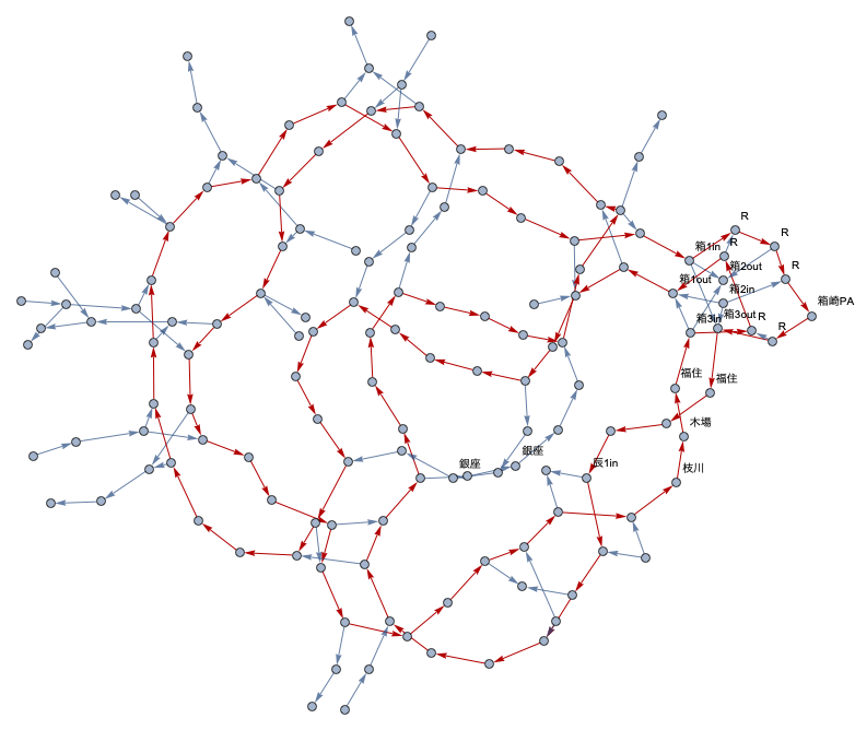
We can find the longest loop way.
HighlightGraph[gg, lg[[77]]]
Red line is a loop found in the center of Tokyo area.

Sorry for Japanese labels in figures, and I don't recommend you to verify the result of loops, actually. Enjoy the virtual tour presented by Mathematica.