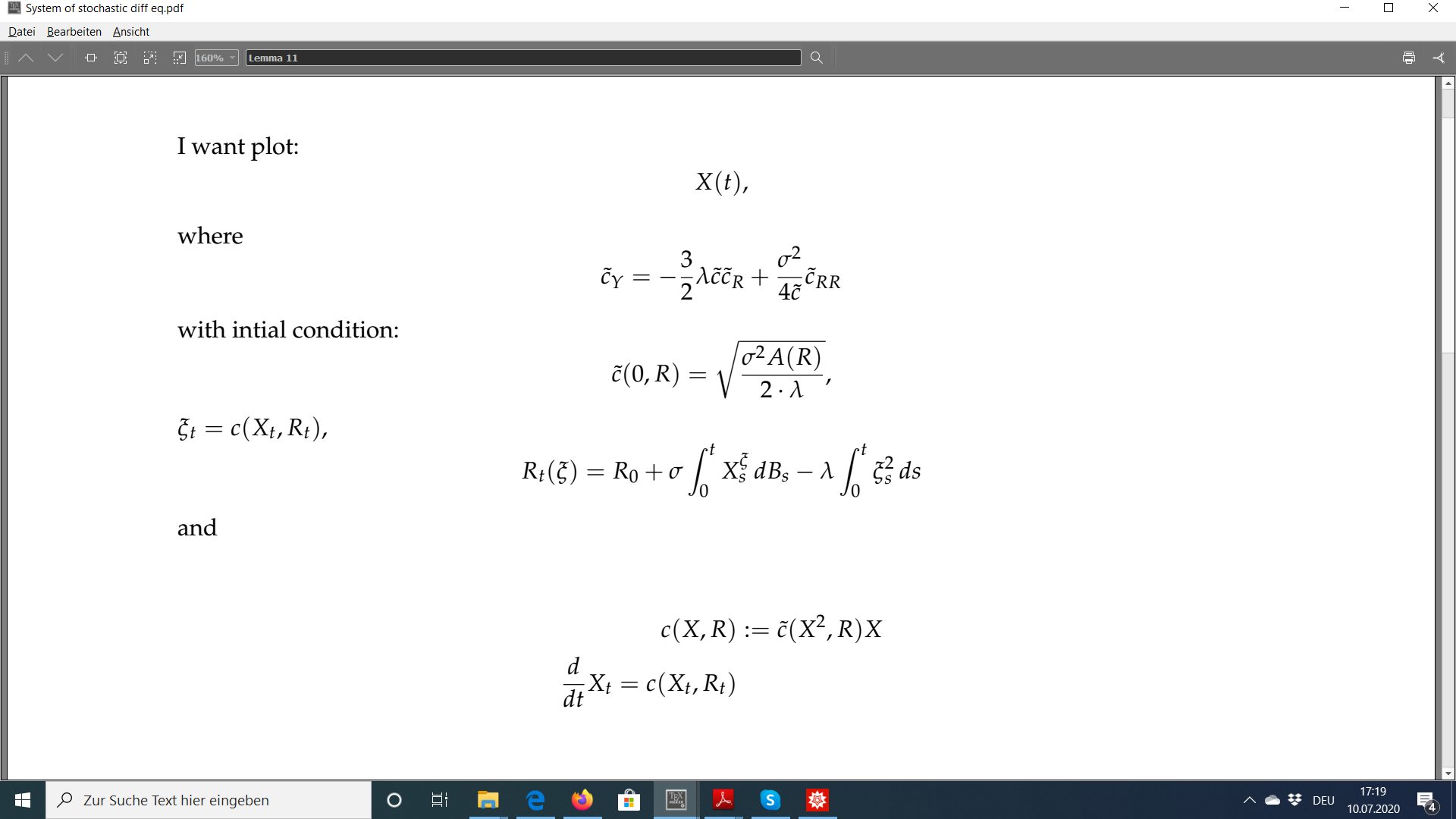
I want to plot X(t) with \lambda = \sigma = x[0] =1 and r[0] = 0.

My code:

pde =  (-3/2) * 1* y[x, t] * D[y[x, t], t] + 1/(4*y[x, t]) * D[D[y[x, t], t], t] - D[y[x, t], x] == 0
sol = NDSolve[{pde, y[0, t] == Sqrt[(1.5 + Tanh[t - 100])^2]}, y[x, t], {x, 0, 1}, {t, 0, 40}] 
f[x_,t_] = y[x, t] /. sol[[1]]
g[x_,t_] = f[x^2, t] * x
proc = ItoProcess[{\[DifferentialD]x[
      t] = -g[x[t], r[t]] \[DifferentialD]t,
             \[DifferentialD] r[t] = - g[x[t], r[t]]^2 \[DifferentialD]t + 
     x[t] \[DifferentialD]W[t]},
            {x [t], r[t]}, {{x, r}, {1, 0}}, t, 
  W \[Distributed] WienerProcess[0, 1]]

My idea is to interpret this as a system of stochastic differential equation.