In the previous reports, Japan case is modeled. In early of this year, Japan national institute confirmed that Japan had infected serially by two major viruses. Following the information, it was found that the case of Japan can be illustrated with the conjunction of two Gompertz curves derived from the differential equation.

US event has been well modeled with a Gompertz curve, however, the difference between the model and reported data becomes non-negligible recently. We can obtain good explanation with the method applied to Japan case.

Principal is straightforward one. First step is to divide the death number trend into the first and second part. Applying Gompertz equation to the first trend and obtain a curve F, then subtract F from the raw trend to obtain second infection trend. Applying Gompertz equation to the second trend which is free from the first infection effect, and obtain a curve L. A curve F+L is the intended answer.

• obtain trend of US data

  country = "US";
  urlCovid19 = "https://pomber.github.io/covid19/timeseries.json"; data \
  = Map[Association, 
    Association[Import[urlCovid19]][
     country], {1}]; ddata = {DateObject[#["date"]], #["deaths"]} & /@ 
    data;
  firstday = ddata[[1, 1]];
  Last[ddata]
  

• get US basic data

  entity = "US";
  population = Normal[Entity["Country", entity]["Population"]]
  

• get data for the estimation

  peeled = Map[{QuantityMagnitude[#[[1]] - firstday], #[[2]]} &, 
     ddata];
  tidyd = Map[First, Gather[peeled, #1[[2]] == #2[[2]] &]];
  ListPlot[tidyd]
  

• get death-number per unit observation period

  i5 = BlockMap[#[[2]] - #[[1]] &, tidyd, 2, 1];
  i6 = Map[(#[[2]]/#[[1]]) &, i5];
  i7 = First[Transpose[Drop[i4, 1]]];
  

• get first part, where dividing report day is set to 155

  i5 = Select[tidyd, #[[1]] <= 155 &];
  

• set initial guess for the first part

  start = 70;
  model0 = n b^Exp[-c ( t - start)];
  initialguess = {n -> 120000, c -> 0.03, b -> 0.02};
  Show[
   Plot[model0 /. initialguess, {t, 0, 1000}, 
    PlotRange -> {{0, 200}, {0, 150000}}],
   ListPlot[i5]
   ]
  

• estimate a Gompertz curve fitted

  ans = FindFit[i5, model0, initialguess /. Rule -> List, t, 
    MaxIterations -> 200]
  

• obtain second part subtracted the effect of first part

  pdays = First[Transpose[tidyd]];
  death = Last[Transpose[tidyd]];
  ListPlot[diff = 
    Transpose@{pdays, death - (model0 /. ans /. t -> pdays)}]
  

• set initial guess of subtracted second part

  start = 145;
  model1 = n b^Exp[-c ( t - start)];
  initialguess = {n -> 40000, c -> 0.05
     , b -> 0.03};
  Show[
   Plot[model1 /. initialguess, {t, 0, 1000}, 
    PlotRange -> {{0, 200}, {0, 40000}}],
   ListPlot[diff]
   ]
  

• get Gompertz curve fitted

  ans3 = FindFit[diff, model1, initialguess /. Rule -> List, t, 
    MaxIterations -> 200]
  
  upto = 220;
  Show[
   ListPlot[diff],
   Plot[model1 /. ans3, {t, 0, upto}, 
    PlotLegends -> 
     Placed[Text[Style["Second invasion", Bold]], {0.32, 0.75}]],
   PlotRange -> {{0, upto}, {0, 40000}}]
  

• calculate percentage of death number

  percent = 
   100 Divide[(model0 /. ans) + (model1 /. ans3) /. ans /. 
      t -> Infinity, population]
  

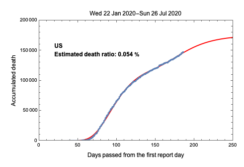
• Finally obtained curve and reported death number of US

  fdate = First[ddata][[1]];
  ldate = Last[ddata][[1]];
  upto = 250;
  
  Show[
   Plot[(model0 /. ans) + (model1 /. ans3), {t, 0, upto}, 
    PlotRange -> {{0, upto}, {0, 200000}}, 
    PlotStyle -> {Red, Thickness[0.005]}],
  
   ListPlot[tidyd, 
    PlotLegends -> 
     Placed[Text[
       Style[country <> "\n" <> "Estimated death ratio: " <> 
         ToString[DecimalForm[percent, 3]] <> " %", Bold]], {0.3, 
       0.75}]],
  
   ImageMargins -> 20,
   Frame -> True,
   PlotLabel -> DateString[fdate] <> "-" <> DateString[ldate],
   FrameLabel -> {Style["Days passed from the first report day", 12], 
     Style["Accumulated death", 12]}, LabelStyle -> {Black}]
  

• Output of the code

Keep in mind that this model is supposed of the virus generic variation in US.