Message Boards Message Boards

0
|
13280 Views
|
39 Replies
|
11 Total Likes
View groups...
Share
Share this post:

Create a color gradient using a variable?

Posted 3 years ago

Let say I have a function

F[x_,y_]:=x^2+6y^(3/2)

Now I want to plot a 2D plot of F[ ] vs x, and need to use y variable as a color gradient. Here I want to vary y as a color axis and the values of F will be plotted against x it will be like thisF vs x but with different function

POSTED BY: John Wick
39 Replies

Hello Rohit, that looks great,

but on my system that doesn't work. I don't know why, there is a Part - Error. Ok, I am using a hand-axe material out of the stone - age.

Part::partw: Part 1 of {} does not exist. >>
Part::pspec: Part specification {}[[1,1]] is neither an integer nor a list of integers. >>

Seems my workaround is not necesaary

POSTED BY: Hans Dolhaine

There seems to be a workaround. Is it this what you want?

data = Table[{Thread[n[s]]}, {s, 20, 100, 1}] /. {a -> 1, 
     Tn -> 0.0005, g -> 10.75, f -> 5.6*10^-9} // Flatten[#, 3] &;
data11 = Table[{Thread[A1[s]]}, {s, 20, 100, 1}] /. {a -> 1, 
     Tn -> 0.0005, g -> 10.75, f -> 5.6*10^-9} // Flatten[#, 3] &;
data = {-3.44558, -3.41357, -3.37737, -3.33768, -3.29502, -3.24983, \
-3.20244, -3.15314, -3.10215, -3.04968, -2.99589, -2.94094, -2.88496, \
-2.82808, -2.7704, -2.71203, -2.65306, -2.59358, -2.53367, -2.47341, \
-2.41287, -2.35212, -2.29122, -2.23024, -2.16923, -2.10824, -2.04733, \
-1.98654, -1.92592, -1.86551, -1.80535, -1.74547, -1.68592, -1.62673, \
-1.56792, -1.50952, -1.45155, -1.39405, -1.33704, -1.28053, -1.22454, \
-1.16909, -1.11419, -1.05987, -1.00612, -0.952961, -0.900404, \
-0.848456, -0.797122, -0.746411, -0.696325, -0.64687, -0.598048, \
-0.549861, -0.502311, -0.455397, -0.409121, -0.363481, -0.318476, \
-0.274104, -0.230361, -0.187246, -0.144754, -0.102882, -0.0616244, \
-0.0209778, 0.0190633, 0.0585042, 0.0973505, 0.135608, 0.173283, 
   0.210381, 0.246909, 0.282874, 0.318282, 0.35314, 0.387454, 
   0.421233, 0.454483, 0.487211, 0.519424};

data11 = {1.01252*10^-9, 1.13838*10^-9, 1.27117*10^-9, 1.41033*10^-9, 
   1.55528*10^-9, 1.70539*10^-9, 1.85999*10^-9, 2.01842*10^-9, 
   2.17996*10^-9, 2.34391*10^-9, 2.50956*10^-9, 2.6762*10^-9, 
   2.84314*10^-9, 3.00971*10^-9, 3.17523*10^-9, 3.33909*10^-9, 
   3.50068*10^-9, 3.65943*10^-9, 3.81481*10^-9, 3.96633*10^-9, 
   4.11354*10^-9, 4.25601*10^-9, 4.39339*10^-9, 4.52533*10^-9, 
   4.65156*10^-9, 4.77183*10^-9, 4.88592*10^-9, 4.99367*10^-9, 
   5.09495*10^-9, 5.18966*10^-9, 5.27775*10^-9, 5.35918*10^-9, 
   5.43394*10^-9, 5.50208*10^-9, 5.56364*10^-9, 5.61871*10^-9, 
   5.66737*10^-9, 5.70975*10^-9, 5.74598*10^-9, 5.77621*10^-9, 
   5.8006*10^-9, 5.81934*10^-9, 5.83259*10^-9, 5.84056*10^-9, 
   5.84344*10^-9, 5.84144*10^-9, 5.83476*10^-9, 5.82362*10^-9, 
   5.80821*10^-9, 5.78876*10^-9, 5.76547*10^-9, 5.73855*10^-9, 
   5.70821*10^-9, 5.67464*10^-9, 5.63805*10^-9, 5.59864*10^-9, 
   5.55659*10^-9, 5.51208*10^-9, 5.4653*10^-9, 5.41643*10^-9, 
   5.36562*10^-9, 5.31305*10^-9, 5.25886*10^-9, 5.20321*10^-9, 
   5.14625*10^-9, 5.0881*10^-9, 5.02891*10^-9, 4.96879*10^-9, 
   4.90787*10^-9, 4.84627*10^-9, 4.78408*10^-9, 4.72141*10^-9, 
   4.65836*10^-9, 4.59502*10^-9, 4.53147*10^-9, 4.4678*10^-9, 
   4.40409*10^-9, 4.34039*10^-9, 4.27679*10^-9, 4.21333*10^-9, 
   4.15009*10^-9};

col = (# - 20)/80 & /@ Table[20 + (j - 1) 80/99, {j, 1, 100}];
dat3 = Transpose[{data, data11}];
rest = {Hue[col[[Position[dat3, #][[1, 1]]]]], Point[#]} & /@ dat3;
rest = rest /. Point[{x_, y_}] -> Point[{x, Log[y]}];


ListLogPlot[{dat3[[1]], dat3[[-1]]}, PlotStyle -> PointSize[.02], 
 PlotRange -> {{-1.5, 1.0}, {10^-12, 10^-8}}, Frame -> True,
 Epilog -> {PointSize[.02], rest}]
POSTED BY: Hans Dolhaine
Posted 3 years ago

Thanks Hans, I think now it is perfect

POSTED BY: John Wick

Hi John, that is fine. Cool.

But I noticed that you have 81 datapoints, but 100 colors.

Length[data]
Length[col]

Is it really that what you intend?

POSTED BY: Hans Dolhaine
Posted 3 years ago

Hi Hans,

On 12.1.1 ColorFunction works for ListPlot so the plot can be generated like this

ListLogPlot[Transpose[{data, data11}],
 PlotStyle -> PointSize[.02],
 PlotRange -> {{-1.5, 1.0}, {10^-12, 10^-8}},
 Frame -> True,
 ColorFunction -> Function[{x, y}, Hue[col[[Position[data, x][[1, 1]]]]]],
 ColorFunctionScaling -> False]

enter image description here

POSTED BY: Rohit Namjoshi
Posted 3 years ago

In the previous example the x values were integers Range[10] so col[[x]] is a valid expression. In this example the x values are reals so col[[x]] is invalid. Rewrite col as an interpolating function that maps the x values to the corresponding value to use for Hue, or perhaps use Rescale.

POSTED BY: Rohit Namjoshi
Posted 3 years ago

Sorry now I have tried the Rescale method and changed

ColorFunction-> Function[{x,y},Hue[Rescale[s,{0,1}]]]

Now there is no part error but still the points are not colored differently, I am getting exactly the same plot as previous without any error.

POSTED BY: John Wick
Posted 3 years ago

The function takes arguments x and y but they are not used in the body of the function. What is s?

POSTED BY: Rohit Namjoshi

Your requests for help are very polite, indeed. Anyhow, that is really strange. Colorfunction seems not to operate on points:

ListPlot[
 Table[{x, x^2}, {x, 0, 4}], PlotStyle -> PointSize[.03],
 ColorFunction -> Function[{x, y}, Hue[.7 x]], 
 ColorFunctionScaling -> False
 ]

but

ListLinePlot[
 Table[{x, x^2}, {x, 0, 4}], PlotStyle -> Thick,
 ColorFunction -> Function[{x, y}, Hue[.7 x]], 
 ColorFunctionScaling -> False
 ]
POSTED BY: Hans Dolhaine
Posted 3 years ago

I have now tried a new problem but colors are not coming properly

data = Table[{Thread[n[s]]}, {s, 20, 100, 
     1}] /. {a -> 1, Tn -> 0.0005, g -> 10.75, 
    f -> 5.6*10^-9} // Flatten[#, 3] &
data11 = Table[{Thread[A1[s]]}, {s, 20, 100, 
     1}] /. {a -> 1, Tn -> 0.0005, g -> 10.75, 
    f -> 5.6*10^-9} // Flatten[#, 3] &
data = {-3.44558, -3.41357, -3.37737, -3.33768, -3.29502, -3.24983,
-3.20244, -3.15314, -3.10215, -3.04968, -2.99589, -2.94094, -2.88496, 
-2.82808, -2.7704, -2.71203, -2.65306, -2.59358, -2.53367, -2.47341, 
-2.41287, -2.35212, -2.29122, -2.23024, -2.16923, -2.10824, -2.04733, 
-1.98654, -1.92592, -1.86551, -1.80535, -1.74547, -1.68592, -1.62673, 
-1.56792, -1.50952, -1.45155, -1.39405, -1.33704, -1.28053, -1.22454, 
-1.16909, -1.11419, -1.05987, -1.00612, -0.952961, -0.900404, 
-0.848456, -0.797122, -0.746411, -0.696325, -0.64687, -0.598048, 
-0.549861, -0.502311, -0.455397, -0.409121, -0.363481, -0.318476, 
-0.274104, -0.230361, -0.187246, -0.144754, -0.102882, -0.0616244, 
-0.0209778, 0.0190633, 0.0585042, 0.0973505, 0.135608, 0.173283, 
0.210381, 0.246909, 0.282874, 0.318282, 0.35314, 0.387454, 0.421233, 
0.454483, 0.487211, 0.519424}

data11 = {1.01252*10^-9, 1.13838*10^-9, 1.27117*10^-9, 1.41033*10^-9, 
 1.55528*10^-9, 1.70539*10^-9, 1.85999*10^-9, 2.01842*10^-9, 
 2.17996*10^-9, 2.34391*10^-9, 2.50956*10^-9, 2.6762*10^-9, 
 2.84314*10^-9, 3.00971*10^-9, 3.17523*10^-9, 3.33909*10^-9, 
 3.50068*10^-9, 3.65943*10^-9, 3.81481*10^-9, 3.96633*10^-9, 
 4.11354*10^-9, 4.25601*10^-9, 4.39339*10^-9, 4.52533*10^-9, 
 4.65156*10^-9, 4.77183*10^-9, 4.88592*10^-9, 4.99367*10^-9, 
 5.09495*10^-9, 5.18966*10^-9, 5.27775*10^-9, 5.35918*10^-9, 
 5.43394*10^-9, 5.50208*10^-9, 5.56364*10^-9, 5.61871*10^-9, 
 5.66737*10^-9, 5.70975*10^-9, 5.74598*10^-9, 5.77621*10^-9, 
 5.8006*10^-9, 5.81934*10^-9, 5.83259*10^-9, 5.84056*10^-9, 
 5.84344*10^-9, 5.84144*10^-9, 5.83476*10^-9, 5.82362*10^-9, 
 5.80821*10^-9, 5.78876*10^-9, 5.76547*10^-9, 5.73855*10^-9, 
 5.70821*10^-9, 5.67464*10^-9, 5.63805*10^-9, 5.59864*10^-9, 
 5.55659*10^-9, 5.51208*10^-9, 5.4653*10^-9, 5.41643*10^-9, 
 5.36562*10^-9, 5.31305*10^-9, 5.25886*10^-9, 5.20321*10^-9, 
 5.14625*10^-9, 5.0881*10^-9, 5.02891*10^-9, 4.96879*10^-9, 
 4.90787*10^-9, 4.84627*10^-9, 4.78408*10^-9, 4.72141*10^-9, 
 4.65836*10^-9, 4.59502*10^-9, 4.53147*10^-9, 4.4678*10^-9, 
 4.40409*10^-9, 4.34039*10^-9, 4.27679*10^-9, 4.21333*10^-9, 
 4.15009*10^-9}

col = (# - 20)/80 & /@ Table[20 + (j - 1) 80 /99, {j, 1, 100}];
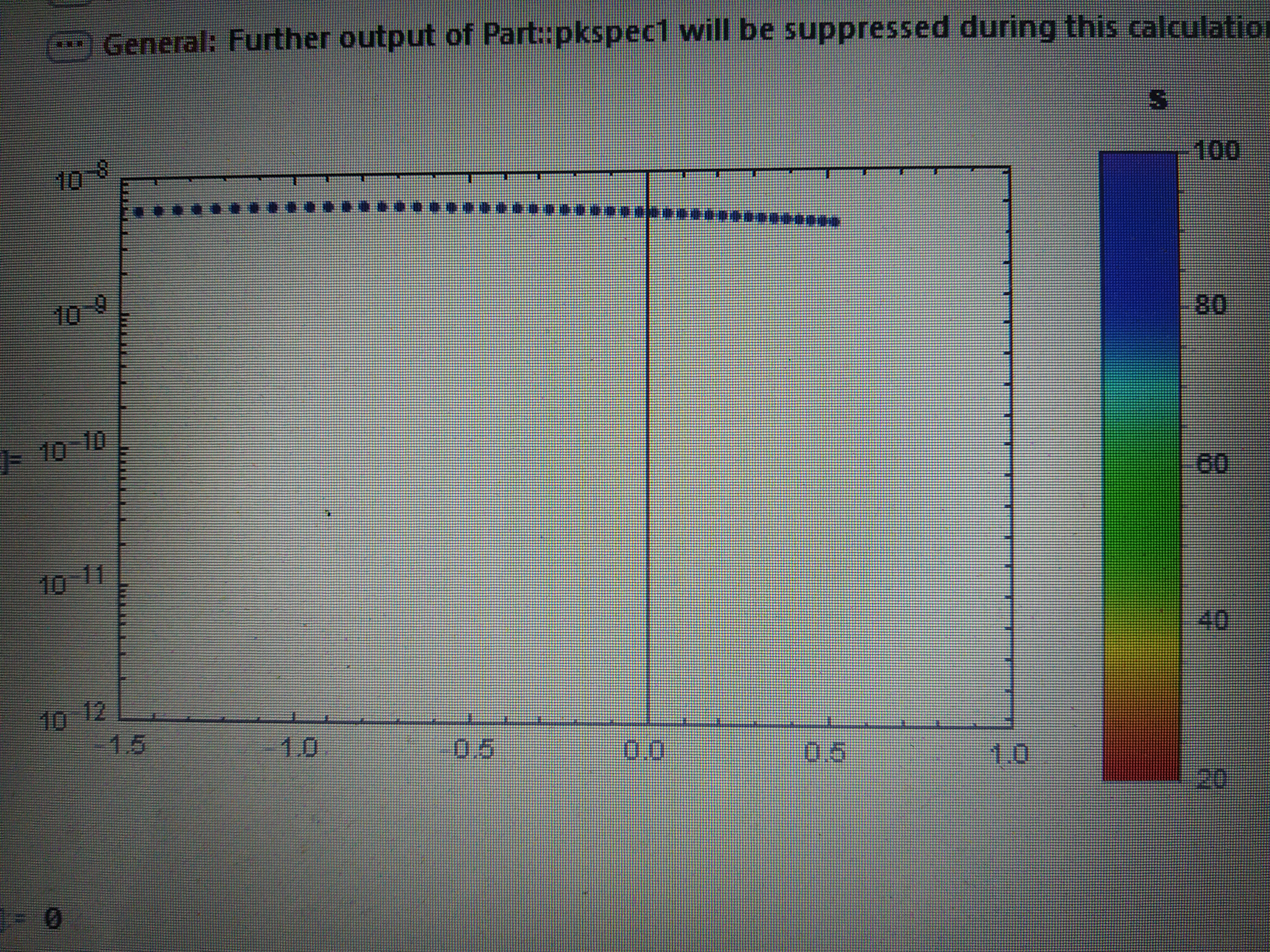
ListLogPlot[Transpose[{data,data11}], PlotStyle -> AbsoluteThickness[3], 
 PlotRange -> {{-1.5, 1.0}, {10^-12, 10^-8}}, 
 ColorFunction -> Function[{x, y}, Hue[0.7 col[[x]]]], 
 ColorFunctionScaling -> False
 , PlotLegends -> 
  BarLegend[{Hue[(# - 20)/100] &, {20, 100}}, 
   LegendLabel -> 
    Style["s", 12, Bold], LegendMarkerSize -> {30, 250}], Frame -> True]
Attachment

Attachments:
POSTED BY: John Wick

And still another method (be sure to calculate sumpt in advance)

ShowLegend[
 ListLinePlot[Transpose[{vn/Tn, sumpt}], PlotStyle -> Thick, 
  ColorFunction -> Function[{x, y}, Hue[.7 col[[x]]]], 
  ColorFunctionScaling -> False, ImageSize -> Large, 
  PlotRange -> {{0, 12}, {0, ub}}, AxesOrigin -> {0, 0}],
 {Hue[.7 (1 - #)] &, 8, "   \!\(\*
StyleBox[\"3.1\",\nFontSize->14]\)", "   \!\(\*
StyleBox[\"1.0\",\nFontSize->14]\)", LegendShadow -> None, 
  LegendSize -> {.18, .8}, LegendPosition -> {.7, -.5}
  }]
POSTED BY: Hans Dolhaine
Posted 3 years ago

That's a lot to learn, Thank you for sharing <3

POSTED BY: Yasmin Hussain

Is there a reason why you have not upgraded to v12?

Well, for me it is simply too expensive. I am retired. And even "if"", I don't like the idea to have to have a download instead of a CD, and that only for one only machine. I use Mathematica on my desktop, and on my laptop, but at different times. So essentially once.

And after all there are lots of functionalities in v7 about which I have no knowledge. I get the impression that the higher versions of Mathematica contain functionalities which are not "really" necessary, and on the other hand , those which are really cool.

And I admire your knowledge of Mathematica and your problem-solving-ability.

POSTED BY: Hans Dolhaine
Posted 3 years ago

Sorry, now I have managed to fix col but the color axis is too thin is it possible to make the color axis by BarLegend.

POSTED BY: John Wick
Posted 3 years ago

Not sure what you mean by 'color axis is too thin`. Do you mean the thickness of the line? If so

PlotStyle -> AbsoluteThickness[5]

If you want a thicker BarLegend then

PlotLegends -> 
 BarLegend[{Hue[(# - 1)/3.1] &, {1, 3.1}}, LegendMarkerSize -> {30, 250}]

{30, 250} is {width, height}

ListLinePlot[Transpose[{vn/Tn, sumpt}],
 PlotStyle -> AbsoluteThickness[5],
 ColorFunction -> Function[{x, y}, Hue[.7 col[[x]]]],
 ColorFunctionScaling -> False,
 PlotLegends -> 
  BarLegend[{Hue[(# - 1)/3.1] &, {1, 3.1}}, LegendMarkerSize -> {30, 250}]]

enter image description here

POSTED BY: Rohit Namjoshi

Hi Rohit: Big Smile! Cool!!

But why does the Legend goes only up to 3.0? (As you may remember I use(still) Mma v7)

POSTED BY: Hans Dolhaine
Posted 3 years ago

Hi Hans,

You did all of the hard work, I just tweaked your code a tiny bit to work with v12.1.1.

The PlotLegends package is deprecated, so I commented out Needs["PlotLegends"]. In v12 BarLegend chooses "nice" values for the ticks, so the legend goes up to 3.1, but only 3.0 has a tick label. I could not find a way to change that.

Is there a reason why you have not upgraded to v12?

POSTED BY: Rohit Namjoshi

And as usual in Mathematica there is another method to generate a Plot (make sure your notebook window is large enough):

Needs["PlotLegends`"]

v = 246
E1 = 9000

Tn = {300, 500, 469, 650, 546, 389, 456, 411, 523, 700}
vn = Range[10] Tn
sumpt = Table[0, {10}]
nn = 1000
Do[rr = RandomReal[{1, 3.1}, 10];
 E1T = E1 vn rr/v;
 PT = E1T/Tn - 7 Log[vn]/Tn + Log[Tn/100];
 sumpt = sumpt + PT, {nn}]
sumpt = sumpt/nn
col = (# - 1)/2.1 & /@ Table[1 + (j - 1) 2.1/9, {j, 1, 10}]
lb = .8 Min[sumpt];
ub = 1.2 Max[sumpt];
ListLinePlot[Transpose[{vn/Tn, sumpt}], PlotStyle -> Thick, 
 ColorFunction -> Function[{x, y}, Hue[.7 col[[x]]]], 
 ColorFunctionScaling -> False,
 ImageSize -> Large,
 PlotRange -> {{0, 12}, {0, ub}},
 AxesOrigin -> {0, 0},
 Epilog -> Inset[
   Graphics[
    Legend[Hue[.7 (1 - #)] &, 8, "3.1", "1.0",
     LegendShadow -> None,
     LegendSize -> {(ub - lb)/3, ub - lb}
     ]], {10.2, lb}, {-1, -1}]
 ]
POSTED BY: Hans Dolhaine
Posted 3 years ago

How to manipulate the col function when working with more than 10 data say 100 data, and also how to change the ub and lb definitions without averaging(i.e. single evaluation, which is the case for me)

POSTED BY: Updating Name

Ok. I spent some more time at the computer. Look at the notebook attached. I hope it is correct and that what you wanted. Note that you can drag the colorscale towards teh line-plot.

Attachments:
POSTED BY: Hans Dolhaine

Ok. State now is: you have all the hints that you should be able to do what you want.

POSTED BY: Hans Dolhaine

Hi John,

didn't you understand? Your code is WRONG, Have you ever run it? I tried to fix the flaws and asked you if you agree to the results of the new version. But you did not answer to that question. So: please check it.

Then ((ETv)/(vnE1)) is the array of the random numbers. Check this too.

After that we can talk about colors.

Here is a 1st attempt

v = 246
E1 = 9000

Tn = {300, 500, 469, 650, 546, 389, 456, 411, 523, 700}
vn = Range[10] Tn
sumpt = Table[0, {10}]
nn = 1000
Do[
 rr = RandomReal[{1, 3.1}, 10];
 E1T = E1 vn rr/ v;
 PT = E1T/Tn - 7 Log[vn]/Tn + Log[Tn/100];
 sumpt = sumpt + PT,
 {nn}]
sumpt = sumpt/nn
col = Table[1 + (j - 1) 2.1/9, {j, 1, 10}]
ListLinePlot[
 Transpose[{vn/Tn, PT}],
 PlotStyle -> Thick,
 ColorFunction -> Function[{x, y}, Hue[col[[x]]]],
 ColorFunctionScaling -> False
 ]
POSTED BY: Hans Dolhaine
Posted 3 years ago

Thanks for giving your valueable time, I think now it is exactly what I needed, but how to assign the correct color axis, and also guide me how to draw the color line in case of log color data(i.e. a log color axis)

POSTED BY: John Wick
Posted 3 years ago

Also I have failed to understand what is the meaning of this part

Do[
 rr = RandomReal[{1, 3.1}, 10];
 E1T = E1 vn rr/ v;
 PT = E1T/Tn - 7 Log[vn]/Tn + Log[Tn/100];
 sumpt = sumpt + PT,
 {nn}]
sumpt = sumpt/nn
col = Table[1 + (j - 1) 2.1/9, {j, 1, 10}]
POSTED BY: John Wick

This is the calculation of averages. The code for PT is executed nn times, the results are added and finally divided by nn. I have no idea whether you wanted such a thing. col is the range of colors.

POSTED BY: Hans Dolhaine

What do you mean by " the correct color axis " ? The colors are coded accroding to the random number used in the calculation fpr the point in question , your ((ETv)/(vnE1)) .

POSTED BY: Hans Dolhaine
Posted 3 years ago

There in the posted image there is a color axis corresponding to the ratio, It is important since it makes the graphics more detailed, the color axis shown in above figure shows how the colors corresponding to each points related to the values of ((ET*v)/(vn*E1))

Secondly, I only want simply the values of PT (for each random number i.e. one point for each set of data, don't need any avg like thing) plotted against vn/Tn

POSTED BY: John Wick

Hi John,

your code gives error messages because of synthax.mistakes. I had a close look at it and concluded that you want to calculate PT and do it like this

v = 246
E1 = 9000

Tn = {300, 500, 469, 650, 546, 389, 456, 411, 523, 700}
vn = Range[10] Tn
E1T = E1 vn RandomReal[{1, 3.1}, 10]/ v
PT = E1T/Tn - 7 Log[vn]/Tn + Log[Tn/100]

Is this right?

But a Plot doesn't look like yours

ListLinePlot[Transpose[{vn/Tn, PT}]]

Any comments?

POSTED BY: Hans Dolhaine
Posted 3 years ago
v = 246
E1 = 9000

PT = ((ET*v)/(
   vn*E1))/((vn/Tn)^-1*(v/
    E1)) - 7*(Log[vn]/Tn) + 
  Log[Tn/100];
vn/Tn= {1, 2, 3, 4, 5, 6, 7, 8, 9, 10};
Tn= {300, 500, 469, 650, 546, 389, 456, 411, 523, 700};
((ET*v)/(vn*E1)) := 
 RandomReal[{1, 3.1}, {10}];

Now I have to plot between (vn/Tn) vs PT making a variable color axis of ((ET*v)/(vn*E1)) as like the attatched graphics( it should look like a set of data points but having varing colors depending on ((ET*v)/(vn*E1))) , The plot may not exactly look like it since I have putted some mannual data by hand

POSTED BY: John Wick

?????????????????????????

What do you want to do?

Perhaps you can give a handmade example?

POSTED BY: Hans Dolhaine
Posted 3 years ago
v = 246
E1 = 9000

PT = ((Subscript[E1, T]*v)/(
   Subscript[v, n]*E1))/((Subscript[v, n]/Subscript[T, n])^-1*(v/
    E1)) - 7*(Log[Subscript[v, n]]/Subscript[T, n]) + 
  Log[Subscript[T, n]/100]
Subscript[v, n]/Subscript[T, n] = {1, 2, 3, 4, 5, 6, 7, 8, 9, 10};
Subscript[T, n] = {300, 500, 469, 650, 546, 389, 456, 411, 523, 700};
((Subscript[E1, T]*v)/(Subscript[v, n]*E1)) = 
 RandomReal[{1, 3.1}, {10}]

Now I have to randomly vary the last ratio to some range and make it the color bar axis and the values for PT and vn/Tn for each ratios can be plotted PT vs vn/Tn plot making the ratio as color axisPlot

POSTED BY: John Wick

OK. But you are merely repeating your words. For me it is not all all clear what you want to do. And: I suggest that you eliminate all these subscript-expressions. They may be a reason for a lot of mistakes

POSTED BY: Hans Dolhaine
Posted 3 years ago

I am now explaining the problem with more detailed way, Let's consider

F[x_,y_]:=Sqrt[ (5*10^-6)*x^2*(5*10^-9)^y]
y=Sqrt[Tan[x]]

Now I have to randomly vary x to some range and make it the color bar axis and the values for F[x,y] and y for each x are plotted in y vs F[x,y]

POSTED BY: John Wick
Posted 3 years ago

I still don't understand the question? What are you asking for? Kind of lost here.

POSTED BY: Yasmin Hussain

Or this?

F[x_, y_] := x^2 + 6 y^(3/2)

Plot3D[F[x, y], {x, -3, 3}, {y, 0, 4}, ColorFunction -> Function[{x, y, z}, Hue[y]] ]
POSTED BY: Hans Dolhaine

Like this? I think you will have to adapt the Hue-expression

Plot[
 Cos[x] Exp[- .1 x^2], {x, -5, 5},
 PlotStyle -> Thick,
 ColorFunction -> Function[{x, y}, Hue[ y]]
 ]
POSTED BY: Hans Dolhaine
Posted 3 years ago
Posted 3 years ago

Hi John,

Not clear what you are asking for. Maybe ContourPlot or DensityPlot?

ContourPlot[f[x, y], {x, -10, 10}, {y, 0, 10},
 Contours -> 10,
 ContourLabels -> All,
 ColorFunction -> "Rainbow",
 PlotRangePadding -> Scaled[.04]]

DensityPlot[f[x, y], {x, -10, 10}, {y, 0, 10},
 ColorFunction -> "Rainbow"]
POSTED BY: Rohit Namjoshi
Posted 3 years ago

I need this type of plot having y as the color variable enter image description here

POSTED BY: John Wick
Reply to this discussion
Community posts can be styled and formatted using the Markdown syntax.
Reply Preview
Attachments
Remove
or Discard

Group Abstract Group Abstract