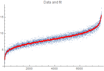
I think you want to make use of Mathematica's time series functions which helps one not only "measure" the noise but also "characterize" the noise.

Given that you have 7,750 observations over time and that the change over time looks relatively smooth, just using a moving average to provide a fit to obtain the residuals (i.e., noise) is probably adequate. (No need to have a bad fit with a small number of parameters in a parametric model.)

fit = MovingAverage[F2, 49];
time = MovingAverage[Range[Length[F2]], 49];
noise = F2[[time[[1]] ;; time[[Length[time]]]]] - fit;

Show[ListPlot[F2, PlotLabel -> "Data and fit"], ListLinePlot[Transpose[{time, fit}], 
  PlotStyle -> {Thickness[0.006], Red}]]

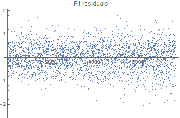
ListPlot[noise, PlotLabel -> "Fit residuals"]

The spread looks relatively uniform across time and one might consider just calculating the variance of the residuals:

Variance[noise]
(* 0.292308 *)

But there might be more structure to the residuals than meets the eye.

tsm = TimeSeriesModelFit[noise]

So the noise might be a bit more complicated than just something proportional to white noise (i.e., uncorrelated normals with variance 0.292308).

To go farther using Time Series methods is what you should consider for characterizing the noise.

I won't confess to a "whim" but anything from 31 and on seems to provide a smooth enough prediction (a prediction much smoother than the observed data). Also using an odd number gets one the appropriate associated time (the middle of the time observations used in the moving average) when constructing the "time" variable using MovingAverage.