Proposal:
Wolfram's mineral database is an interesting resource. In this work I will explore and account for the different chemical elements that are part of each mineral to perform an analysis as a whole. Here, the quantities of each element in each mineral will not be addressed, but only the different atomic elements in each mineral. Also, here in this work I exclude minerals that are formed by only 1 chemical element, that is, I consider only compound minerals. The analysis is done in two parts, the first part is an analysis without taking into account the water that may or may not be in the mineral, that is, the mineral completely dehydrated (only its composition that is linked by covalent bonds etc), the second part I analyze the minerals together with the water. In addition to having obtained a ranking of chemical elements in relation to all available minerals, in the end I get a percentage of how many minerals have oxygen and how many minerals have associated water in their composition.
Database:
Of course, Wolfram's minerals database does not have all the minerals that exist, but it has a very decent amount, where we can make a very representative analysis. First we take the list of minerals in the database and calculate the number of entities:
minerals = EntityList[Entity["Mineral"]];
Length@minerals

Now we will associate each mineral with its chemical formula and, also obtain all the atomic symbols. This operation can take 2 to 3 hours to complete the download from Wolfram's servers:
formulas = Map[#["Formula"] &, minerals];
symbols =
  Map[#["AtomicSymbol"] &, EntityList[EntityClass["Element", All]]];
To quickly make this information available for later use, we can save the data as an .mx file with the help of DumpSave:
filepath = FileNameJoin[{NotebookDirectory[], "formulas.mx"}];
filepath2 = FileNameJoin[{NotebookDirectory[], "symbols.mx"}];
DumpSave[filepath, {formulas}];
DumpSave[filepath2, {symbols}];
Quit[]
That way we can retrieve the data for fast use whenever we want, using Get:
SetDirectory[NotebookDirectory[]];
Get["formulas.mx"]
Get["symbols.mx"]
The definition of “symbols” below:
symbols

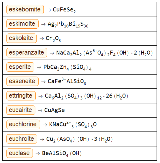
Below is a simple function to have each mineral associated with its chemical formula in an easy way to visualize:
threadFormula[m_, n_] :=
  Thread[minerals[[m ;; n]] -> formulas[[m ;; n]]] //
   Grid[Partition[#, 1], Frame -> All, Alignment -> Left] &;

threadFormula[1000, 1010]
Data Excluding Water:
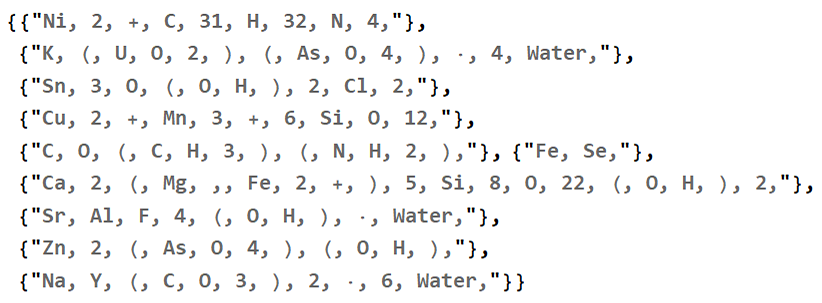
Unfortunately the mineral formulas in the database are in a very complicated format to manipulate, as part is in String, part in Superscript, etc ... so we need to modify and alter the data in an intelligent way to obtain the formulas in a more computable form, at the same time we exclude water associated with minerals that have it:
a1 = {StringDelete[StringDelete[ToString[#], "{"], "}"]} & /@
   Table[Flatten@Apply[List, i, All], {i, formulas}];
a2 = Table[
   StringDelete[
    a1[[x]], {"(, H, 2, O, )", "H, 2, O",
     " ScriptBaselineShifts" ~~ __}], {x, 1, Length@a1}];

a2[[;; 10]]

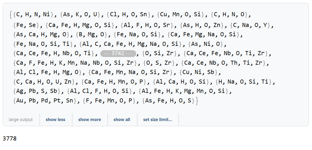
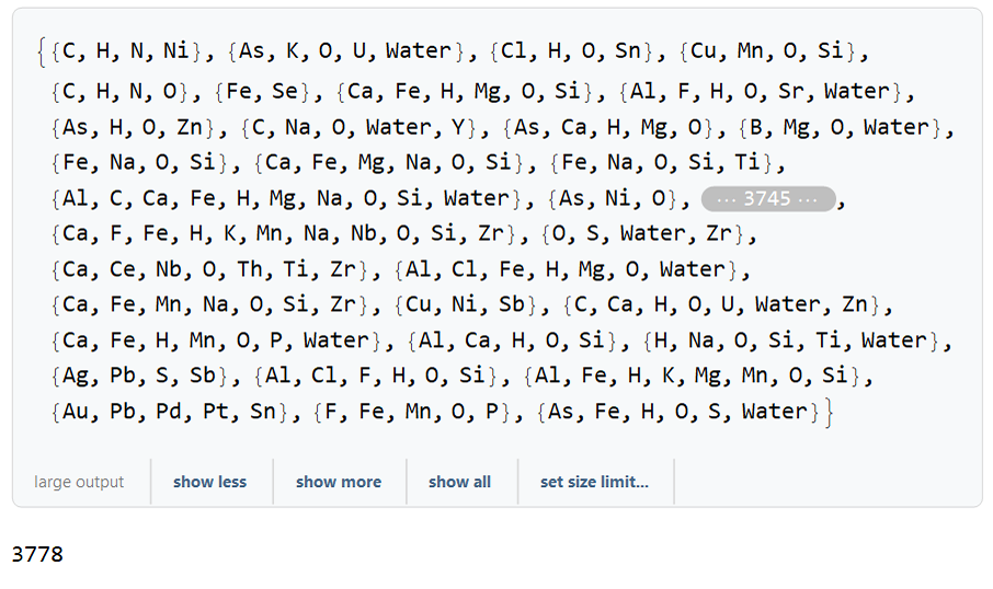
Now extracting the different chemical elements for each mineral and excluding the minerals formed by just one chemical element. Note that the number of minerals went from 3878 to 3778:
a3 = Union[#] & /@
   Flatten[StringCases[#, ReverseSortBy[symbols, Length]] & /@ a2, 1];
a4 = Table[If[Length@a3[[z]] > 1, a3[[z]], Nothing], {z, 1, Length@a3}]
Length@a4
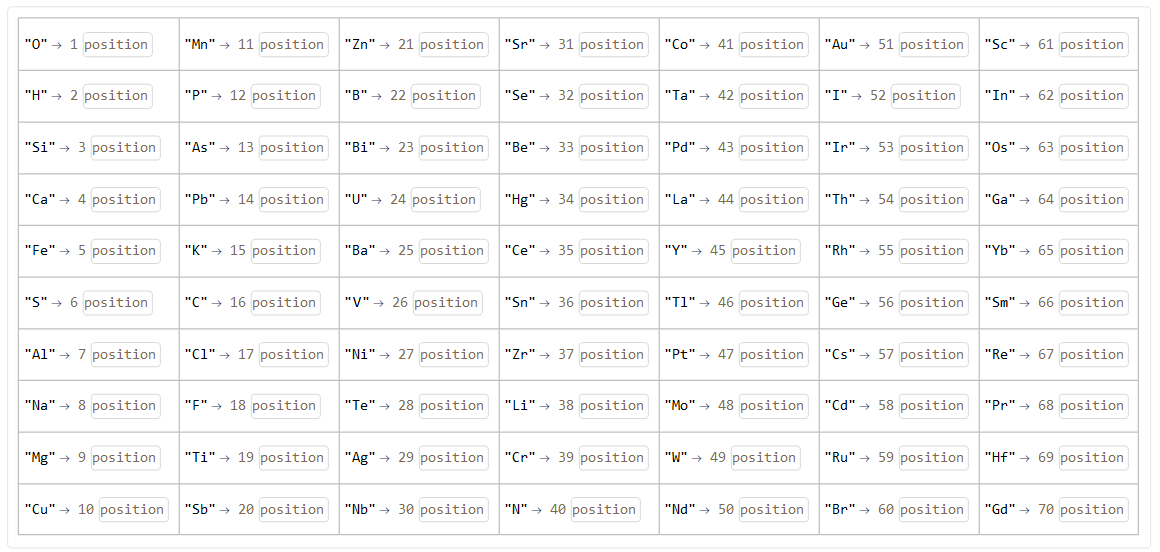
Finally, we can count the composition of different atomic elements that are part of all the minerals in the database. We can see that there are 70 different elements in this list:
a5 = Association[Reverse@SortBy[Normal@Counts@Flatten@a4, Last]]
Length@a5

We can set up a Dataset with the elements and their position (ranking) that are part of all minerals for better visualization:
Transpose[
  Partition[
   Keys@# ->
      Quantity[Position[Normal@a5, #][[1, 1]],
       IndependentUnit["position"]] & /@ Normal@a5 , 10]] // Dataset
For the next parts of this work we have to define the two rules below:
rule1 = Thread[Flatten[Position[symbols, #] & /@ symbols] -> symbols];
rule2 = Join[{0 -> "Water"}, rule1];
With some manipulation of the data, we can for example reorganize the elements in the order they are in the periodic table, that is, in the order of the atomic number, as well as other useful lists to create some graphs and analyzes:
b1 = Table[{Sort[Thread[{Keys@a5, Values@a5}]][[x,
     1]], {Sort[Thread[{Keys@a5, Values@a5}]][[x, 2]]}}, {x, 1,
    Length@a5}];
b2 = Table[
   Entity["Element", b1[[x, 1]]]["AtomicNumber"], {x, 1, Length@b1}];
b3 = SortBy[Table[{b2[[x]], b1[[x, 2, 1]]}, {x, 1, Length@b2}], First];
b4 = Association@
   Table[(b3[[x, 1]] /. rule1) -> b3[[x, 2]], {x, 1, Length@b3}];
b5 = Table[{b3[[x, 1]] /. rule1, b3[[x, 2]]}, {x, 1, Length@b3}];
b4

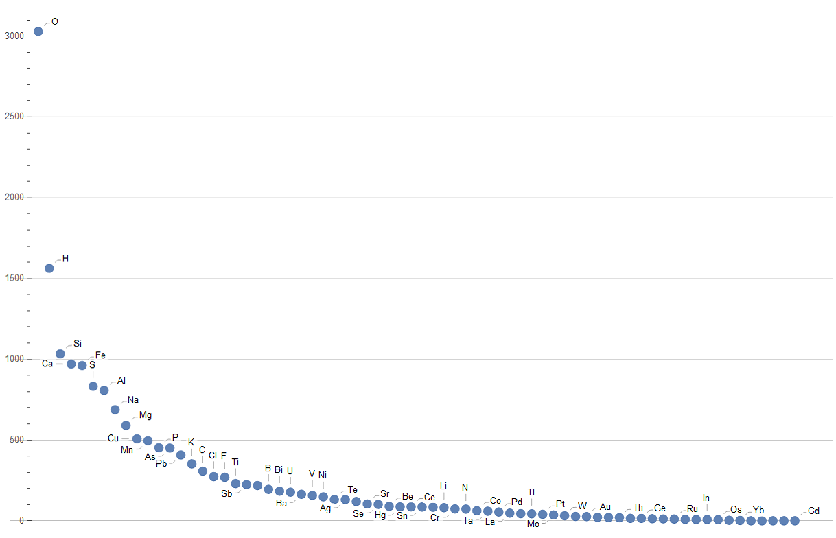
The first plot we have is the different chemical elements that form all the minerals in decreasing order of quantity in which they appear in the whole:
ListPlot[Tooltip /@ a5, ImageSize -> 1000, PlotRange -> All,
 Axes -> {None, Automatic}, GridLines -> {None, Automatic}]
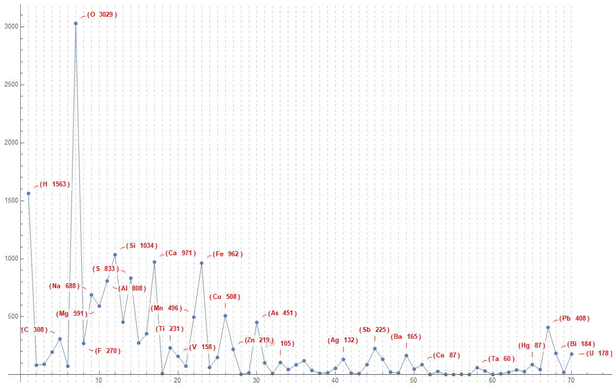
The next plot is the different chemical elements that make up all the mineral samples, but in the order of atomic number. This visualization is interesting because it relates to the periodic table:
ListLinePlot[
 Callout[#[[2]], Style[{#}, 10, Red, Bold], CalloutStyle -> Red] & /@
  b5, ImageSize -> 1000, PlotRange -> All,
 PlotMarkers -> {Automatic, Scaled[0.01]},
 GridLines -> {Table[{x, Dashed}, {x, 1, 70}], None},
 PlotStyle -> Thin]
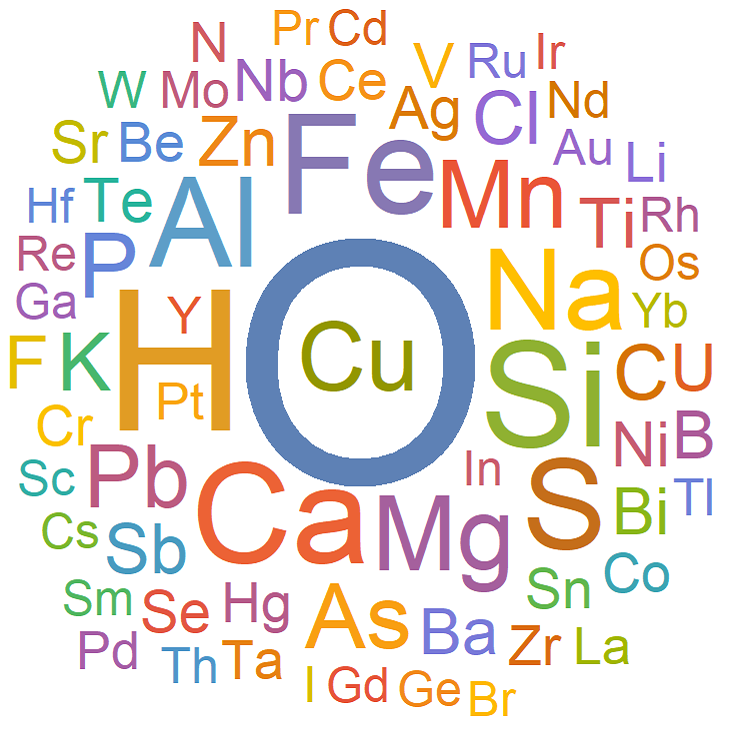
We can view it also in the form of WordCloud:
WordCloud[b5, ImageSize -> Large]
Result of Oxygen:
To conclude the initial analysis, we can see in how many percent of the minerals that there is oxygen attached to the molecular structure in relation to all minerals. We see that this value can reach up to 80%:
"OxygenInTotal" -> Quantity[N[100*b4["O"]/Length@a4], "Percent"]

Data with Water:
With some differences in relation to the first part of this work, instead of excluding water, we can define a new water entity to be included in the formula of the minerals that contain it:
a2W = Table[
   StringReplace[
    a1[[x]], {"(, H, 2, O, )" -> "Water", "H, 2, O" -> "Water",
     " ScriptBaselineShifts" ~~ __ -> ""}], {x, 1, Length@a1}];

a2W[[;; 10]]
With a similar code, with only a few differences, we do the same extraction of atomic symbols plus water in each mineral. Again, we exclude minerals formed by only 1 chemical element:
a3W = Union[#] & /@
   Flatten[StringCases[#,
       ReverseSortBy[Join[symbols, {"Water"}], Length]] & /@ a2W, 1];
a4W = Table[
  If[Length@a3W[[z]] > 1, a3W[[z]], Nothing], {z, 1, Length@a3W}]
Length@a4W
And, again with some manipulation of the data, we created lists and associations to have the result in quantities (including water). Some of these definitions will also be used below to have some plots:
a5W = Association[Reverse@SortBy[Normal@Counts@Flatten@a4W, Last]];
a5W
Length@a5W
b1W = Table[{Sort[Thread[{Keys@a5W, Values@a5W}]][[x,
     1]], {Sort[Thread[{Keys@a5W, Values@a5W}]][[x, 2]]}}, {x, 1,
    Length@a5W}];
b2W = Table[
    Entity["Element", b1W[[x, 1]]]["AtomicNumber"], {x, 1,
     Length@b1W}] /. {Missing[
      "UnknownEntity", {"Element", "Water"}] -> 0};
b3W = SortBy[Table[{b2W[[x]], b1W[[x, 2, 1]]}, {x, 1, Length@b2W}],
   First];
b4W = Association@
   Table[(b3W[[x, 1]] /. rule2) -> b3W[[x, 2]], {x, 1, Length@b3W}];
b5W = Table[{b3W[[x, 1]] /. rule2, b3W[[x, 2]]}, {x, 1, Length@b3W}];
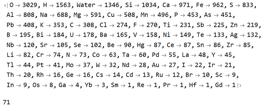
The water being included together with the decreasing order of the amounts of different chemical elements that are part of all minerals:
ListPlot[Tooltip /@ a5W, ImageSize -> 1000, PlotRange -> All,
 Axes -> {None, Automatic}, GridLines -> {None, Automatic}]

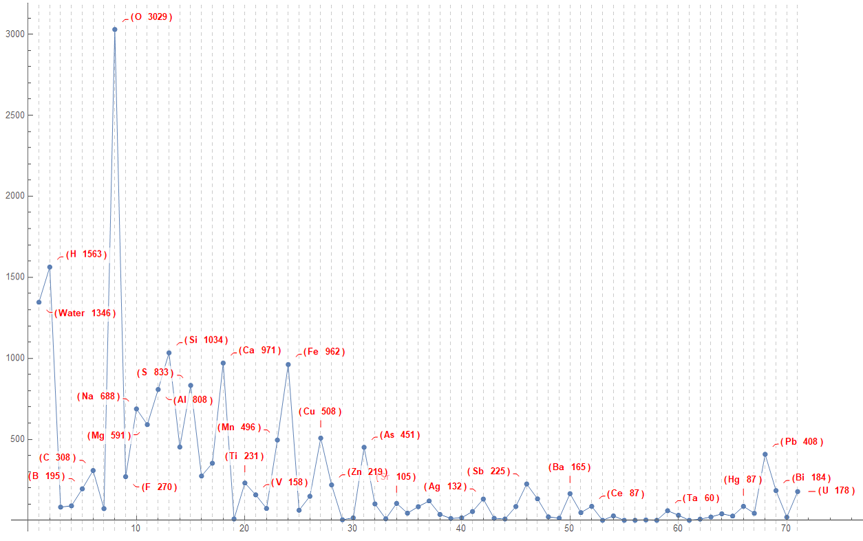
A plot similar to that of the first part of the work, in ascending order of atomic number, but including water and it appears before hydrogen (water defined as position 0) just for viewing:
ListLinePlot[
 Callout[#[[2]], Style[{#}, 10, Red, Bold], CalloutStyle -> Red] & /@
  b5W, ImageSize -> 1000, PlotRange -> All,
 PlotMarkers -> {Automatic, Scaled[0.01]},
 GridLines -> {Table[{x, Dashed}, {x, 1, 71}], None},
 PlotStyle -> Thin]
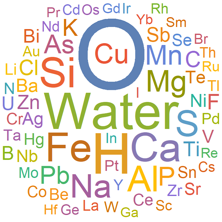
Visualization using WordCloud including water:
WordCloud[a5W, ImageSize -> Large]
Result of Water:
In the way below we calculate how many percent of minerals have water associated with its composition in relation to all available minerals. We can see that an expressive part of them have water (hydrated minerals), more than 1/3 of them:
"WaterInTotal" -> Quantity[N[100*a5W["Water"]/Length@a4W], "Percent"]

Conclusion and Notes:
It is worth mentioning that there may be some flaws in the exclusion and inclusion of water in the calculations, as for example, some organic minerals and some others may be erroneously influenced by the rules stipulated in this work. But it is a minority of these minerals, so although there is some variation in these percentages the value is satisfactorily approximate.
In the future it would be interesting to also analyze the amounts of each chemical element in minerals and not only an analysis as presented here that only counts the different chemical elements. It proved difficult to do this type of analysis because the mineral formulas are in a complex format for computability.
My personal opinion is: it is very interesting that in most minerals we can extract oxygen and water (more from the first than the second) with some physical-chemical treatment, sometimes this can be done in a simple way, sometimes in a complex way, but it demonstrates how there is enough oxygen and water inside the earth's crust, and not only coming from the oceans, from the very formation of our planet.
Thanks.