Message Boards Message Boards

An unexpected effect of Simplify on plotting surfaces

Posted 3 years ago

I have a quadratic equation with complex coefficients. The coefficients depend on two real variables r and w. This quadratic equation has two complex roots, which also depend on two variables r and w. I try to plot the dependence of the absolute value of the root on the variables r and w.

Suddenly I noticed that the surface quality depends on whether I am using expression simplification. Moreover, the more simplifications, the worse the quality.

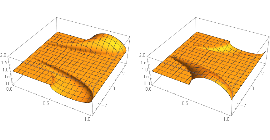
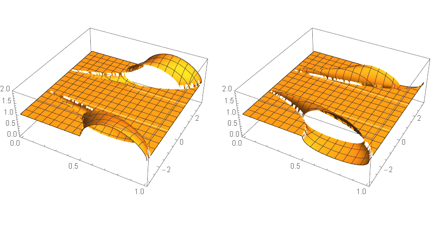
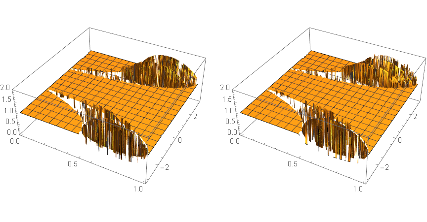
Below, the quadratic roots are simplified in three different ways and three pairs of surfaces correspond to these three ways. Surface quality decreases, build time increases.

My problem is that my project deals with thousands of similar equations and the project code is over 4000 lines. I have used Simplify in many places without fear, and the result is thought-provoking.

Can anyone comment please?

eq=6*q^2*Exp[-3/2*I*w] + q(2r-3)(3(r-3)r(Exp[1/2*I*w]-Exp[-1/2*I*w])+(r-2)(r-1)(Exp[-3/2*I*w]-Exp[3/2*I*w]))-6Exp[3/2*I*w];

sq1=q/.Solve[eq==0,q];
sq2=q/.Solve[Simplify[eq]==0,q];
sq3=Simplify[sq1];

SetOptions[Plot3D,PlotPoints->60,PlotRange->{0,2}];

Timing[g1=GraphicsRow[{Plot3D[Abs[sq1[[1]]],{r,0,1},{w,-Pi,Pi}],Plot3D[Abs[sq1[[2]]],{r,0,1},{w,-Pi,Pi}]},ImageSize->Large]]  [[1]]
Timing[g2=GraphicsRow[{Plot3D[Abs[sq2[[1]]],{r,0,1},{w,-Pi,Pi}],Plot3D[Abs[sq2[[2]]],{r,0,1},{w,-Pi,Pi}]},ImageSize->Large]]  [[1]]
Timing[g3=GraphicsRow[{Plot3D[Abs[sq3[[1]]],{r,0,1},{w,-Pi,Pi}],Plot3D[Abs[sq3[[2]]],{r,0,1},{w,-Pi,Pi}]},ImageSize->Large]]  [[1]]

g1
g2
g3

Below are the results:

Image g1

Image g2

image g3

POSTED BY: Andrey Solovjev
6 Replies

Don't be sad, this is simply what happens when inexact arithmetic meets a discontinuity. For example

x1 = -1 - .0000000000000000000000000000000000000001 I;
x2 = -1 + .0000000000000000000000000000000000000001 I;
Abs[x1 - x2]
Sqrt[x1]
Sqrt[x2]

In your case you can bypass the problem with a simplification that eliminates complex numbers from the radicand:

sq3 = sq1 /. Sqrt[smthg_] :>
   Sqrt[FullSimplify[smthg, Element[w, Reals]]]
Plot3D[Abs[sq3[[2]]], {r, 0, 1}, {w, -Pi, Pi},
 PlotRange -> All, PlotPoints -> 60]
POSTED BY: Gianluca Gorni

Yes, I quite understand that jumping from one root to another, or jumping between sheets of a multi-sheet function, is behind the jumps when drawing surfaces. But, it is very sad that the Mathematics cannot investigate the behavior of a function in space if there are complex numbers somewhere inside the function. It is also disappointing that modification the form of the expression (not the expression itself) had such large consequences.

POSTED BY: Andrey Solovjev

There are at least a couple of underlying issues. One is that the results shown are a very natural consequence of machine arithmetic, in particular for evaluations on branch cuts. That much is a matter of numerical analysis and has essentially nothing to do with the workings of Mathematica. The important point is that, in this situation, form differences should be expected to have consequences. One must thus plan accordingly. One way to improve on it is by using bignum precision in Plot. Below I reuse an example to show that arbitrary precision arithmetic manages better in this ill-conditioned example.

sqs = {sq1[[1]], sq3[[1]], sq1[[2]], sq3[[2]]} /. {r -> 9/10, w -> Pi + 3/10};
{N[sqs], N[sqs, 20]}

(* Out[665]= {{-1.40758 - 0.679938 I, -0.576028 - 
   0.278253 I, -0.576028 - 0.278253 I, -1.40758 - 
   0.679938 I}, {-1.4075784895084728311 - 
   0.6799379196099996129 I, -1.4075784895084728311 - 
   0.6799379196099996129 I, -0.57602825716558496620 - 
   0.27825336756212492578 I, -0.57602825716558496620 - 
   0.27825336756212492578 I}} *)

Another issue is that there is no way (of which I am aware) to use Root objects in quadratic solutions. These typically have better numeric evaluation properties than radical expressions.

POSTED BY: Daniel Lichtblau

I mean, the numerical noises have an imaginary component, because expression under square root is complex, although it simplifies symbolically to a real number.

POSTED BY: Gianluca Gorni

Your sq variables contain a square root of a real quantity. When this quantity becomes negative, the numerical methods become ustable, because the complex square root is discontinuous along the negative real axis. Your three versions of sq are equivalent symbolically, but when evaluated in floating point numbers they generate different small numerical noises that are amplified by the discontinuity.

POSTED BY: Gianluca Gorni

The first two need not agree because Solve can return roots in forms that agree as an ensemble, but not individually, for all possible substitutions of values. This arises when solution branches cross.

The first and third should agree.

eq = 6*q^2*Exp[-3/2*I*w] + 
   q (2 r - 
      3) (3 (r - 3) r (Exp[1/2*I*w] - Exp[-1/2*I*w]) + (r - 2) (r - 
         1) (Exp[-3/2*I*w] - Exp[3/2*I*w])) - 6 Exp[3/2*I*w];

sq1 = q /. Solve[eq == 0, q];
sq3 = Simplify[sq1];
Simplify[sq3 - sq1]

(* Out[641]= {0, 0} *)

But clearly they do not.

In[645]:= {sq1[[1]], sq3[[1]], sq1[[2]], sq3[[2]]} /. {r -> .9, 
  w -> -Pi + .3}

(* Out[645]= {-0.576028 - 0.278253 I, -1.40758 - 0.679938 I, -1.40758 - 
  0.679938 I, -0.576028 - 0.278253 I} *)

This is a bit of a mystery, and might indicate a bug somewhere.

POSTED BY: Daniel Lichtblau
Reply to this discussion
Community posts can be styled and formatted using the Markdown syntax.
Reply Preview
Attachments
Remove
or Discard

Group Abstract Group Abstract