I guess this is a standard example for the use of residues! The function

f[z_] := Exp[z]*Cos[Pi*z]/(z^2 + z)

has two poles:

poles = Solve[z^2 + z == 0, z]
(*  Out:  {{z\[Rule]-1},{z\[Rule]0}}  *)

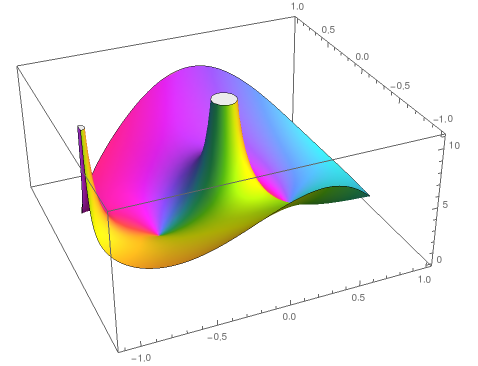
The one at z=-1 is on the contour:

ComplexPlot3D[f[z], {z, -1.1 - 1 I, 1 + 1 I}, RegionFunction -> (Abs[#] <= 1 &), BoxRatios -> {Automatic, Automatic, 1}]

The respective residues are:

Residue[f[z], {z, #}] & /@ {0, -1}
(*  Out:   {1,1/\[ExponentialE]}   *)

So - according to residue theorem - we find for the line integral along Abs[z]==1 (the residue on the pole counts half!):

2 Pi I (1 + 1/(2 E))

But Mathematica can actually handle those integrals directly; because of the pole on the contour the option PrincipalValue -> True is needed:

Integrate[f[Exp[I \[Phi]]] I Exp[I \[Phi]], {\[Phi], 0, 2 Pi}, PrincipalValue -> True]
(*  Out:   \[ImaginaryI] (2+1/\[ExponentialE]) \[Pi]  *)

Counting the residue at the pole on the contour itself seems to require a bit of justification, ...

Well, yes! But the pole in question is of first order, the path of integration is sufficiently well behaving, and in those cases the calculation (I think / I learned at school) is that simple. Or do you disagree with the result?

It should be emphasized that this path integral actually is divergent, and only exists in the sense of a principal value integration.

Am I missing something -- didn't you neglect to insert the dz multiplier after the parameterization?

Definition (or formula from a theorem) of contour integral of complex function $f(z)$ over a contour $C$: let $\gamma: [a, b] \rightarrow \mathbb{C}$ be a parameterization of $C$. Then $\int_C f(z) dz = \int _a^b f(\gamma(t)) \gamma'(t) dt$.

Your expression for the integral seems to be missing the factor $ \gamma'(t)$, which for $\gamma(t) = 0.5 e^{i t}$ should be $0.5 i e^{i t}$.

I suspect that Wolfram|Alpha cannot directly evaluate a contour integral, but that you will have to do the first step yourself, namely, parameterizing the contour (in the standard way?), etc.

Please use spaces and parentheses to clarify the complex function. For example, does piz mean Pi z? And does the formula involve Exp[z] or Exp[z Cos[Pi z]]?

Also, do you mean to integrate around the circle Abs[z]==1?

Did you try to parametrize the circle and reduce the line integral to an ordinary integral (of a complex-valued function of a real variable)?

Is the denominator z^2 + 2 or z^2 + z?