The interesting pattern @Jim Baldwin observed has most likely to do with the number of gray levels induced by aliasing; if this number of gray levels is plotted against rotation this becomes obvious:

xrimg = Table[{x, ImageRotate[img, x]}, {x, 0, Pi, Pi/100}];
ListLinePlot[{#1, (Length@*DeleteDuplicates@*Flatten@*ImageData)[#2]} & @@@ xrimg, PlotRange -> All]

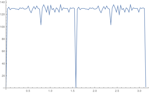
So I guess one should work here with binarized images only.

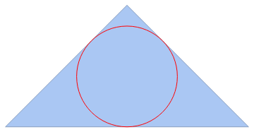
But my main point here is that I was in a way wrong in my post above: This method is not suitable to calculate caliper width! One can easily see this in the following example, where the diameter of the circle by no means has anything to do with caliper:

But nevertheless this method can be useful if the true shape is used instead of the convex hull, and if one no longer concentrates on "caliper" but more on a term like "belly". That gives me my modified routine:

bellyWidth[img_Image] := Module[{borderPts, order, baktMesh},
  borderPts = ImageValuePositions[Thinning[EdgeDetect[Binarize[img]]], 1];
  order = First@FindCurvePath[borderPts];
  baktMesh = MeshRegion[Polygon@borderPts[[order]]];
  -2. NMinValue[SignedRegionDistance[baktMesh, {\[FormalX], \[FormalY]}], {\[FormalX], \[FormalY]}  \[Element] baktMesh]]

Lets check:

rimg = Table[ImageRotate[img, x], {x, 0, Pi, Pi/25}];
{#, bellyWidth[#]} & /@ rimg

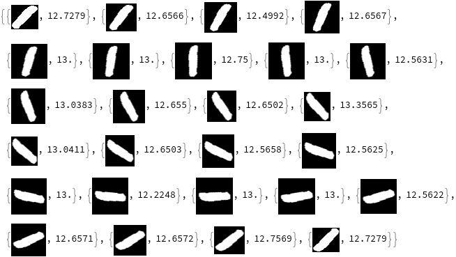
The discrepancies now are (far) below one pixel.

That really reduces the variability. I wonder if the variability/bias could be reduced more by taking an average of a set of arbitrary rotations? I say this because there does seem to be a pattern:

rimg = Table[{x, ImageRotate[img, x]}, {x, 0, Pi, Pi/100}];
t = {#[[1]], caliperWidth[#[[2]]]} & /@ rimg;
ListPlot[t, Joined -> True]

I suspect it is not just the differences; if I am not mistaken, the results ("CaliperWidth" == smallest diameter of the convex hull) seem to be wrong altogether. You can see this simply like so:

Manipulate[Labeled[Show[img, Graphics[{Red, Line[pts]}], ImageSize -> Large], 
  EuclideanDistance @@ pts], {{pts, {{20, 20}, {10, 10}}}, Locator}]

Indeed, seems to be a bug. A little bit difference is expected due to grayscales when you rotate and so on. But should be ~2px max. "CaliperLength" seems to work properly.

I will submit it as a bug.