This is a physics problem that I have found to be very interesting and challenging to implement in Mathematica, I hope some of you have a few good ideas to try.
I want to generate and plot a set of magnetic domains (in 2D) in a ferromagnet, and then have them grow/shrink in response to an applied field (via a Manipulate command). Generally speaking, the image I want to create would look like this.

My approach is to generate a set of space filling, non-overlapping polygons and feed them to Graphics. My very rough solution currently involves making the polygons by hand, and then using Scale to shrink/expand them, i.e.
domains = {{{0, 70}, {0, 50}, {20, 50}, {23, 55}, {23, 70}}, {{23, 70}, {23, 55}, {40, 50}, {40, 70}}, {{40, 70}, {40, 50}, {42, 45}, {70, 50}, {70, 70}}, {{70, 37}, {70, 70}, {95, 70}, {95, 60}, {85, 40}}, {{95, 70}, {100, 70}, {103, 62}, {95, 60}}, {{100, 70}, {140, 70}, {140, 50}, {103, 62}}, {{103, 62}, {140, 50}, {140, 30}, {130, 30}, {115, 45}}, {{95, 60}, {103, 62}, {115, 45}, {100, 40}, {97, 42}}, {{85, 40}, {95, 60}, {97, 42}, {90, 30}}, {{70, 30}, {70, 37}, {85, 40}, {90, 30}, {90, 27}}, {{42, 45}, {70, 50}, {70, 30}, {65, 25}, {37, 24}, {35, 28}}, {{18, 42}, {20, 50}, {23, 55}, {40, 50}, {42, 45}, {35, 28}, {30, 30}}, {{0, 50}, {20, 50}, {18, 42}, {10, 30}, {0, 25}}, {{18, 42}, {30, 30}, {10, 30}}, {{0, 0}, {0, 25}, {10, 30}, {30, 30}, {35, 28}, {37, 24}, {37, 15}, {5, 0}}, {{5, 0}, {37, 15}, {42, 0}}, {{42, 0}, {37, 15}, {37, 24}, {65, 25}, {70, 0}}, {{70, 0}, {65, 25}, {70, 30}, {90, 27}, {97, 10}, {95, 0}}, {{90, 27}, {90, 30}, {97, 42}, {100, 40}, {105, 18}, {97, 10}}, {{105, 18}, {100, 40}, {115, 45}, {130, 30}}, {{95, 0}, {97, 10}, {105, 18}, {130, 30}, {140, 30}, {140, 0}}};
d1 = Cos[RandomReal[{0, 2 \[Pi]}, 21]];
Graphics[{
EdgeForm[Black], FaceForm[], Arrowheads@Small,
Table[{FaceForm[Blend[{Red, Blue}, .5 (d1[[ii]] + 1)]],
Scale[Polygon[domains[[ii]]], 0.5 d1[[ii]] + 1, Mean[domains[[ii]]]],
Translate[Rotate[Scale[Arrow[{{-1, 0}, {1, 0}}], 5], ArcCos[d1[[ii]]]], Mean[domains[[ii]]]]}, {ii, dd}],
{Thick, EdgeForm@Black, Rectangle[{0, 0}, {140, 70}]}
}, PlotRange -> {{0, 140}, {0, 70}}]
Unfortunately, this doesn't work as gaps will form between some of the shrunken domains, and the overlapping expanded domain boundaries look non-physical, i.e. can be concave.
I have stumbled on two methods to generate the domains programatically.
1. Based on the Mathematica documentation, this method produces bitmapped imaged of random domains. It looks really nice, but doesn't lend itself for use in a Manipulate based demo (I think).
aa = Graphics[{
Green, Rectangle[{0, 0}, {20, 20}], Black, Point[RandomReal[{2, 18}, {10, 2}]]
}];
bb = ColorQuantize[ImageAdjust@LaplacianGaussianFilter[DistanceTransform[aa], 2], 20]

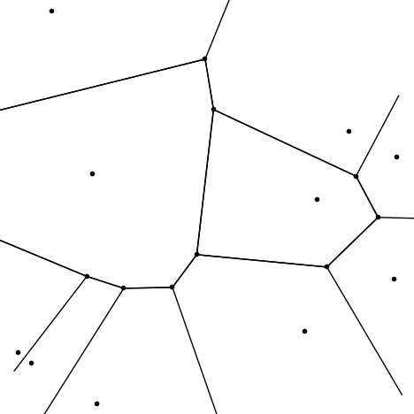
2. Also based on Mathematica documentation, generate the random domains using the Computational Geometry package,
pp = RandomReal[{2, 18}, {10, 2}];
{vorvert, vorval} = VoronoiDiagram[pp];
DiagramPlot[pp, vorvert, vorval, LabelPoints -> False, TrimPoints -> 4]
The polygon information is stored in vorvert and vorval.

this method looks promising for generating and plotting the random domain polygons, but I am left with the issue of how to grow/shrink the domains properly. In principle, this can be done by moving the edges of the domains aligned with the field in the direction of the field, i.e. if the applied field is horizontal, then the vertical (or close to vertical) edges of the relevant polygons would move to the left/right.
Any thoughts as to how this process (or even the initial generation of the domains) can be done efficiently enough (i.e. computationally fast) enough to put in a Manipulate command and have it be very responsive.
Finally, a big thanks to S. M. Blinder who's demo
http://demonstrations.wolfram.com/MagneticHysteresis/ gave me the inspiration for this problem.