Hello. I have some questions on how to implement propperly the KL expansion in mathematica using KarhunenLoeveDecomposition.
I have constructed the matrix realizationMat. it contains 101 measurements of 90 Gaussian stochastic processes. I implement the expansion as
VA1 = realizationMat[[1]];
VA2 = realizationMat[[2]];
KLVariablesB = KarhunenLoeveDecomposition[{VA1, VA2...}]
However, I have problems understanding the output. In the documentation it says:
rows of the transformation matrix m are the eigenvectors of the covariance matrix formed from the arrays ai.
yet, if I plot rows of m as ListPlot[{KLVariablesB[[2, 1]]}, Joined -> True] I obtain what can be seen in figure 1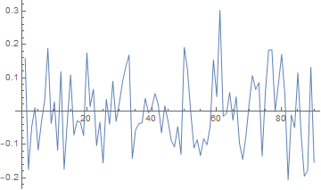 .
.
Another quote from the documentation is
The transformed arrays bi are uncorrelated, are given in order of decreasing variance, and have the same total variance as ai.
As far as I know, this means that these are the random variables defined in the theory. However, if I plot them, These don't look like random variables, as can be seen in figure 2: 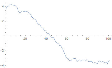 . These look like eigenvectors but aren't Gaussian eigenvectors, being my data Gaussian.
Can someone please tell me if there is something wrong with my data or why the eigenvectors don't look like eigenvectos and the random variables don't look like random variables?
Best regards. jaime.
E. G. I will attach the code I am using in case someone wants to take a look.
 Attachments:


