The GKL Cellular Automaton can be defined by a 32-digit hexadecimal code (Table 4.1), which determines a 128-digit binary genome on change of base:

FromHexCode[gen_] := PadLeft[IntegerDigits[FromDigits[ToExpression[
     Characters[gen] /. {"f" -> 15, "e" -> 14, "d" -> 13, "c" -> 12, 
       "b" -> 11, "a" -> 10}], 16], 2], 128]
GKLHex="005f005f005f005f005fff5f005fff5f";
GKLBin=FromHexCode[GKLHex]; 

The binary genome satisfies an interesting invariant transformation property, which reveals inherent parity+inversion symmetry:

SortTup = Tuples[{0, 1}, 7];
InverseParity = Flatten[Position[SortTup, 
           Reverse[#] /. {0 -> 1, 1 -> 0}] & /@ SortTup];
SymCheck[gen_]:= Tally[Subtract[gen, gen[[InverseParity]] /. {0 -> 1, 1 -> 0}]]
SymCheck@GKLBin
Out[]:={{0, 128}}

A more direct definition is given in terms of a linear functional acting on 128 of the 7-digit vectors which form the rule space:

GKLBin2 = With[{LF = {0, 0, 0, 1, 1, 0, 1}},
  Sign[If[#[[4]] == 1, LF.#,
       Reverse[LF].#] & /@ (SortTup /. {0 -> -1})] /. {-1 -> 0}]
SameQ[GKLBin, GKLBin2]
Out[]:=True

According to the definition by linear functional, the symmetry property is guaranteed. After reversing all rule vectors and fliping their bits, and after applying the same two linear functionals, the sign of the output value must also flip. This is true for any chosen linear functional, and there are other known good examples, mentioned elsewhere.

The parity+inversion transformation property suggests an analogy that allows us to formulate a good majority classifier in two dimensions. Going from Parity symmetry, to cyclic C4 symmetry, suggests that we use four symbols rather than 2. Here is a basic definition of the Linear Functional (actually it's slightly more complicated than that, so read the code):

RuleTable[gen_] := With[{ind = Flatten[Position[gen, 1]]}, {
    {0, n_, w_, s_, e_, ne_, nw_, sw_, se_} :> 
     With[{com = Commonest[{0, n, w, s, e, ne, nw, sw, se}[[ind]] ]}, 
      If[Length[com] == 1, com[[1]], 0]],
    {1, n_, w_, s_, e_, ne_, nw_, sw_, se_} :> 
     With[{com = Commonest[{1, w, s, e, n, nw, sw, se, ne}[[ind]] ]}, 
      If[Length[com] == 1, com[[1]], 1]],
    {2, n_, w_, s_, e_, ne_, nw_, sw_, se_} :> 
     With[{com = Commonest[{2, s, e, n, w, sw, se, ne, nw}[[ind]] ]}, 
      If[Length[com] == 1, com[[1]], 2]],
    {3, n_, w_, s_, e_, ne_, nw_, sw_, se_} :> 
     With[{com = Commonest[{3, e, n, w, s, se, ne, nw, sw}[[ind]] ]}, 
      If[Length[com] == 1, com[[1]], 3]]
    }];

RuleDepict[gen_] :=  ArrayPlot[
  ReplaceAll[gen, {c_, n_, w_, s_, e_, ne_, nw_, sw_, se_} :> {
     {nw, n, ne}, {w, c, e}, {sw, s, se}}], ImageSize -> 50]

C4Classifier = {0, 1, 1, 0, 0, 0, 0, 0, 1};
RuleDepict[C4Classifier]

With a few more functions we can make interesting animations:

RandInit[n_] := Partition[RandomSample[Flatten[
    MapIndexed[Table[#2 - 1, -Subtract @@ #1] &,
     Partition[Append[Prepend[Sort@RandomSample[
          N[1 - (2 Range[n^2]/n^2 - 1)^2] -> Range[n^2]
          , 3], 0], n^2], 2, 1], 1]]], n]

Update2D[RT_, init_] := With[{len = Length@init},
  Table[{init[[i, j]],
     init[[i, Mod[j + 1, len] /. {0 -> len} ]],
     init[[Mod[i - 1, len] /. {0 -> len}, j ]],
     init[[i, Mod[j - 1, len] /. {0 -> len} ]],
     init[[Mod[i + 1, len] /. {0 -> len}, j ]],
     init[[Mod[i + 1, len] /. {0 -> len} , 
      Mod[j + 1, len] /. {0 -> len} ]],
     init[[Mod[i - 1, len] /. {0 -> len} , 
      Mod[j + 1, len] /. {0 -> len} ]],
     init[[Mod[i - 1, len] /. {0 -> len} , 
      Mod[j - 1, len] /. {0 -> len} ]],
     init[[Mod[i + 1, len] /. {0 -> len} , 
      Mod[j - 1, len] /. {0 -> len} ]]
     } /. RT, {i, 1, len}, {j, 1, len} ]]

    Fitness[gen_, inits_] := Total[Map[
       If[Count[Flatten@Evo[gen, #, (Length@inits[[1]])^2][[-1]],
           Commonest[Flatten@#][[1]] ] == (Length@inits[[1]])^2, 1, 0] &,
       inits]]

Evo[gen_, init_, ngen_] := 
 NestWhileList[Update2D[RuleTable[gen], #] &, init, UnsameQ, All, ngen]

Depict[cond_] := 
 ArrayPlot[cond, 
  ColorRules -> {0 -> White, 1 -> Red, 2 -> Blue, 3 -> Green}]

Now for the fun part:

dat = Evo[C4Classifier, RandInit[50], 50^2];
Commonest[Flatten[dat[[1]]]] == Union[Flatten[dat[[-1]]]]
ListAnimate[Depict /@ dat]

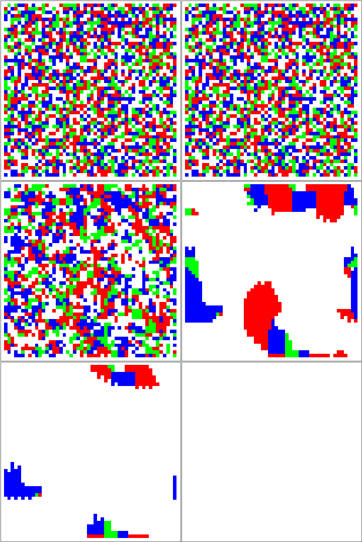
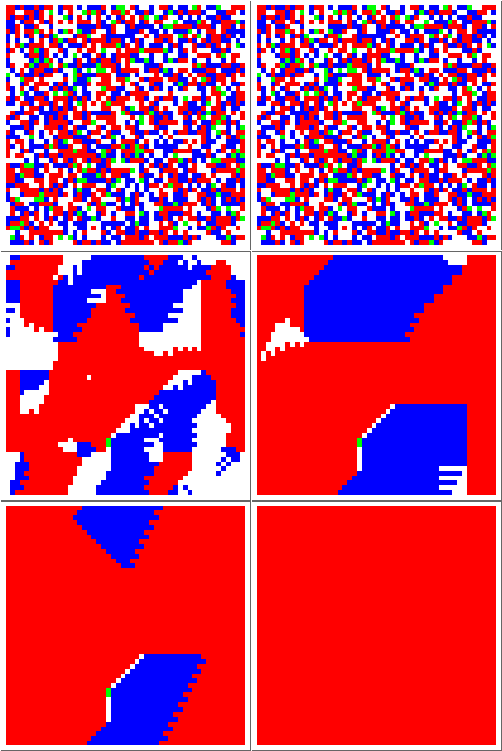
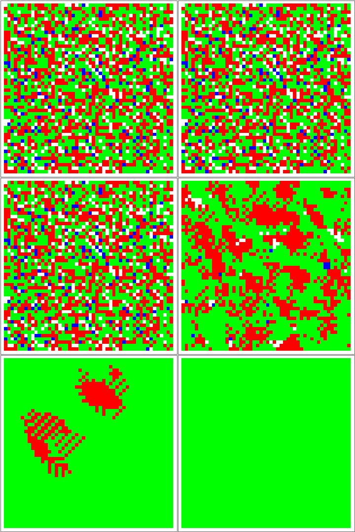
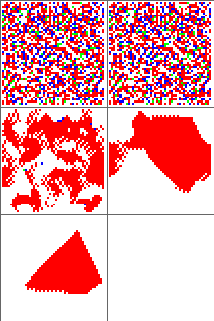
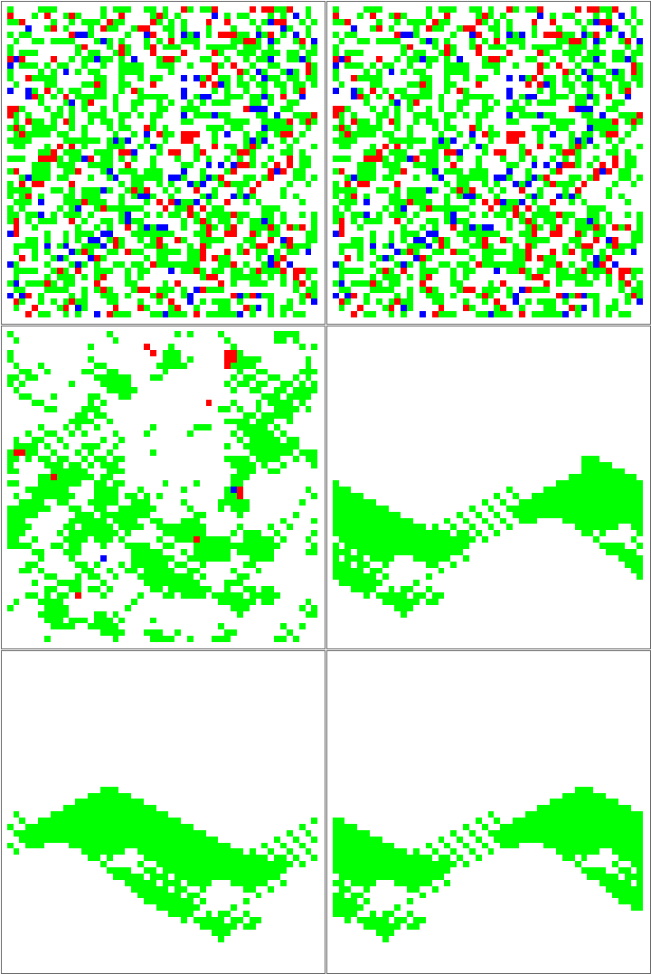
There are some obvious similarities to 1D-GKL classifier, so perhaps in the future more analysis will be done to characterize behavior and possibly find better classifiers. The space of possibilities is immensely huge, so genetic algorithms will need some intelligence when searching.