Message Boards Message Boards

1
|
19087 Views
|
8 Replies
|
9 Total Likes
View groups...
Share
Share this post:

Image Compression

Posted 11 years ago
Hi!!

I need a code (or pseudocode) of mathematica to compress a picture of  n x m pixels.

Input a Jpeg

compress the jpeg

and export jpeg then and before compressed

Please help me.

Thanks!!
POSTED BY: Graphics Wolfram
8 Replies

Hi there! Just use image resize and increase the size of the picture about forty times (40), and then save the picture with the size increases in an image folder of the windows...I don t know why but the file size for the picture decreases from 2MB to 45k...

Posted 11 years ago
Now I see that correct handling of JPG information is impossible in Mathematica without re-implementing of the built-in Importing and Exporting subroutines for JPG.
POSTED BY: Alexey Popkov
I wouldn't say "correct". JPEG is not a representation it is a lossy compression algorithm, thus the command "Save as JPEG" equals to "delete some infomation". But it is a mystery for me why the option "CompressionLevel" -> 0 results in a file which is larger than the original.

For example, we can compare the Shennon entropy for the original and Mathematica processed images:
image[1] = Import["http://i.stack.imgur.com/ZhYwB.jpg"];
image[2] = Import[Export["test.jpg", Import["http://i.stack.imgur.com/ZhYwB.jpg"], "CompressionLevel" -> 0]];
entopies[1] = N@Entropy[Join @@ #] & /@ Transpose[Round@RGBtoYCbCr[image[1]], {2, 3, 1}];
entopies[2] = N@Entropy[Join @@ #] & /@ Transpose[Round@RGBtoYCbCr[image[2]], {2, 3, 1}];
The results are pretty much the same.
entopies[1]/entopies[2]
(* {0.999987, 1.00002, 0.999851} *)
The Shannon entropy (up to constant factor) is the approximate length of  Huffman coding data, which is the main part of JPEG-file.
POSTED BY: Grisha Kirilin
Posted 11 years ago
When saying "correct" I had in mind making incremental changings in a JPG file. For example, I wish to make a lossy compression for a part of a JPG image without loosing any information in another part. I know that it is theoretically possible only for blocks of pixels in the JPG file, but this possibility is very interesting.
POSTED BY: Alexey Popkov
I do not understand the first and the second part of the code: RGB to YCbCr and Inverse transform

My level of mathematica is too bad...

Is not there an easier way?

Thanks!
POSTED BY: Graphics Wolfram
Hi,

you can use JPEG itself! Here is my code, but I make no efforts to optimize it thus it can be really slow. First of all, you need define RGB to YCbCr transform. I found very nice code here via Mr.Wizard (up to some small correction):
 With[{v1 = Developer`ToPackedArray@{16`, 128`, 128`},
   m1 = Developer`ToPackedArray@{{65.481, 128.553,
       24.966}, {-37.797, -74.203, 112`}, {112`, -93.786, -18.214}}},
  RGBtoYCbCr[a : {_, _, _}?VectorQ] := v1 + m1.a;
  RGBtoYCbCr[img_Image] := RGBtoYCbCr@ImageData[img(*,"Byte"*)];
  RGBtoYCbCr[a_ /; MatchQ[Dimensions@a, {_, 3}]] :=
   Transpose[v1 + m1.Transpose[a]];
  RGBtoYCbCr[a_ /; MatchQ[Dimensions@a, {_, _, 3}]] :=
   Transpose[v1 + m1.Transpose[a, {2, 3, 1}], {3, 1, 2}];]

Inverse transform:
 With[{v1 = Developer`ToPackedArray@{-16`, -128`, -128`},
   m1 = Developer`ToPackedArray@
     Inverse@{{65.481, 128.553, 24.966}, {-37.797, -74.203,
        112`}, {112`, -93.786, -18.214}}},
  YCbCrtoRGB[a : {_, _, _}?VectorQ] := m1.(a + v1);
  YCbCrtoRGB[a_ /; MatchQ[Dimensions@a, {_, 3}]] :=
   Transpose[m1.(Transpose[a] + v1)];
  YCbCrtoRGB[a_ /; MatchQ[Dimensions@a, {_, _, 3}]] :=
   Transpose[m1.(Transpose[a, {2, 3, 1}] + v1), {3, 1, 2}];]
Then it is necessary to define the Fourier discrete cosine transform.
fnorm = Developer`ToPackedArray@
   Normal@SparseArray[{{1, 1} -> 1, {i_, i_} -> Sqrt[2]}, {8, 8}];
bnorm = Developer`ToPackedArray@
   Normal@SparseArray[{{1, 1} -> 1, {i_, i_} -> 1/Sqrt[2]}, {8, 8}];

ForwardDCT[matrix_] := fnorm.FourierDCT[matrix - 128, 2].fnorm;
BackwardDCT[matrix_] := 128 + FourierDCT[bnorm.matrix.bnorm, 3];
Please, notice the JPEG uses DCT in slightly different way than Wolfram Mathematica. Next step is to define the quntization tabels for all channels:
 DQT["luma"] =
   Developer`ToPackedArray@{{16, 11, 10, 16, 24, 40, 51, 61}, {12, 12,
      14, 19, 26, 58, 60, 55}, {14, 13, 16, 24, 40, 57, 69, 56}, {14,
      17, 22, 29, 51, 87, 80, 62}, {18, 22, 37, 56, 68, 109, 103,
      77}, {24, 35, 55, 64, 81, 104, 113, 92}, {49, 64, 78, 87, 103,
      121, 120, 101}, {72, 92, 95, 98, 112, 100, 103, 99}};
 
 DQT["chroma"] =
   Developer`ToPackedArray@{{17, 18, 24, 47, 99, 99, 99, 99}, {18, 21,
     26, 66, 99, 99, 99, 99}, {24, 26, 56, 99, 99, 99, 99, 99}, {47,
     66, 99, 99, 99, 99, 99, 99}, {99, 99, 99, 99, 99, 99, 99,
     99}, {99, 99, 99, 99, 99, 99, 99, 99}, {99, 99, 99, 99, 99, 99,
     99, 99}, {99, 99, 99, 99, 99, 99, 99, 99}};
The last step is the quntization itself:
Quantization[channel_, block_, quality_] :=
  BackwardDCT[
   quality DQT[channel] Round[
     ForwardDCT[block]/(quality DQT[channel])]];
Now, we can start. Import an image and divide it into 8*8 blocks:
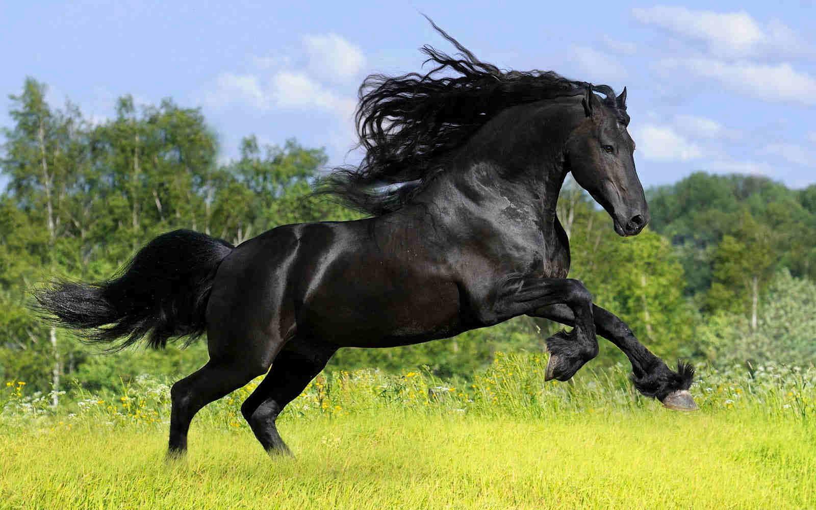
horse = Import["http://i.stack.imgur.com/ZhYwB.jpg"]
blocks = Partition[#, {8, 8}] & /@
   Transpose[RGBtoYCbCr@horse, {2, 3, 1}];

Then we need to choose the quality of the output.
quality = 2;
Notice that the quality should be large than 1 and quality=1 reduces the size of the output file by factor 1.8. Thus we put a really terrible quality. The next step is quantization of each channel:
 luminance[1] =
   Join @@ (Join @@@ Transpose[#, {2, 1, 3}] & /@
      Map[Quantization["luma", #, quality] &, blocks[[1]], {2}]);
 chrominance[1] =
   Join @@ (Join @@@ Transpose[#, {2, 1, 3}] & /@
      Map[Quantization["chroma", #, quality] &, blocks[[2]], {2}]);
 chrominance[2] =
   Join @@ (Join @@@ Transpose[#, {2, 1, 3}] & /@
      Map[Quantization["chroma", #, quality] &, blocks[[3]], {2}]);
This part works really slow, hence please try to optimize it. The last step is to convert to RGB and save to disk:
SetDirectory[NotebookDirectory[]];
Export["horse.jpg",
Image[YCbCrtoRGB@
   Transpose[{luminance[1], chrominance[1], chrominance[2]}, {3, 1,
     2}]]]
The size of the output file is 2.2 times smaler then initial one. The Mathematica file is attached to this post.
Attachments:
POSTED BY: Grisha Kirilin
Posted 11 years ago
Hi Grisha, thank you for the code!
I think that it is worth to point out that Export to "JPG" uses lossy compression with "CompressionLevel" -> 0.25 by default. So just Importing and then Exporting the image I get 34% smaller JPG file. It would be very interesting to see the results of your compression algorithm without this additional lossy compression by Export. I have tried to Export with  "CompressionLevel" -> 0 but it gives a file which is larger than the original. It raises the question: it is possible in Mathematica to Import a JPG file as Image object and then re-create original file from this Image object (assuming that original file contains no EXIF information)?
POSTED BY: Alexey Popkov
Hi Alexey,

I think it is not possible in a general case. The problem is that different programs, devices and cameras use their own quantization tables (DQT). It is even possible to recognize camera producer by DQT used (DQT is a part of JPEG file). For example Adobe Photoshop uses 12 unique different quantization tables for each channel, e.g., for the luminance they look as follows:

It seems that Mathematica's Import does not take into account (or store) DQTs. Of course, Mathematica uses its own DQT, thus the result will be always differnt from the original, with only one exception — the original picture was created by Mathematica:
SetDirectory[NotebookDirectory[]]
Export["test.jpg", Import["http://i.stack.imgur.com/ZhYwB.jpg"]]
Export["test1.jpg", Import["test.jpg"]]
The sizes of test.jpg and test1.jpg are equal.
POSTED BY: Grisha Kirilin
Reply to this discussion
Community posts can be styled and formatted using the Markdown syntax.
Reply Preview
Attachments
Remove
or Discard

Group Abstract Group Abstract