This was suggested by the video created by Alex Kontorovich that accompanies his article " How I loved to Love and Fear the Riemann Hypothesis," Quanta Magazine, January 4, 2021.
https://www.quantamagazine.org/how-i-learned-to-love-and-fear-the-riemann-hypothesis-20210104
It is a much simpler version of the reproduction of that video made by Clayton Shonkwiler in this community post
https://community.wolfram.com/groups/-/m/t/2154374
which I had not seen before posting this. First, a cover function for
ParametricPlot[ReIm[f], ...]
to provide an obviously missing object from the current, limited, supply of built-in functions for visualization of complex functions.
ComplexParametricPlot[f_, {u_, umin_, umax_},
  opts : OptionsPattern[]] :=
 ParametricPlot[ReIm[f], {u, umin, umax},
  Evaluate@FilterRules[{opts}, Options[ParametricPlot]]]
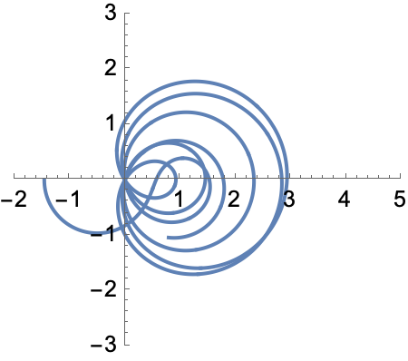
Now we move complex variable z = 1/2+t I along the critical line of the Riemann zeta functions, tracing out a curve in the complex plane, Each time the curve passes through the origin we have reached another zero of the zeta function.
Manipulate[
 ComplexParametricPlot[Zeta[1/2 + s I], {s, 0, t},
  PlotRange -> {{-2, 5}, {-3, 3}}, PerformanceGoal -> "Quality"],
 {{t, 1, "t"}, 0.99, 101, Appearance -> "Labeled"}]
Here's a snapshot:
(I thank Mark Normand for pointing me to the Quanta Magazine article suggesting this kind of visualization. It's possible this is a standard kind of visualization of location of zeros, but I had not run into it before.)


