Update post

Hi all,

Thank you so much for taking a crack at this!! There are a few complicating factors I abridged out of the original post for brevity. For example, I'm going to be dealing with spin diffusion across material interfaces, i.e. the edge of a membrane in contact with water, and therefore there will be different values of the diffusivity D/a^2 at different points on the grid. This is no big deal to implement though. I have begun coding a solution inspired by all of yours (@Hans Dolhaine; @Henrik Schachner; Joshua Schrier), that basically iteratively operates on the 1D magnetization. I have had to reach out to the author of the FORTRAN code I'm trying to replicate to ask a few questions about the setup, and am waiting for a reply. When I (hopefully, God willing) finish a full solution, I will verify some prior experimental results and make a new Community Forum post and link it here.

Also, sorry for the delay. In my defense, I'm writing my doctoral thesis and this probably won't make it in; it's a for-the-joy-of-it endeavor!

Gratefully,

Madeleine Sutherland

Dear all,

I do hope that this is not off-topic, but I would like to make the remark that when the evolution of magnetization is described by the respective differential equation (instead of a difference equation), this system can be solved in an analytic way easily:

dim = 10;  (* number of magnets: *)
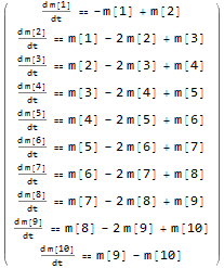
(* definition of the before mentioned "update matrix": *)
mat = Normal@
   SparseArray[{Band[{1, 1}] -> -2, Band[{1, 2}] -> 1, Band[{2, 1}] -> 1}, {dim, dim}];
mat[[1, 1]] = mat[[dim, dim]] = -1;
mat // MatrixForm

Then we have equation : d magVec / dt == mat.magVec, and mat.magVec gives the desired terms (all constants are set to 1) :

(* general magnetic vector: *)
magVec = Table[m[n], {n, 1, dim}];
(* 'd/dt' on lhs is just "symbolic" to show the system of equations! *)
Thread[(d /dt) magVec == mat.magVec] // MatrixForm

(* solution matrix in time 't': Exp[mat t], i.e.: *)
expMat = MatrixExp[mat  t];
(* initial condition - magnetic state at t==0: *)
startMagnVect = Prepend[ConstantArray[0, dim - 1], 1];
(*  {1, 0, 0, 0, 0, 0, 0, 0, 0, 0}  *)
(* analytical solution: *)
mgt = expMat.startMagnVect;
mgtN = N[mgt];

Plot of the result, i.e. magnetization in time:

labels = Style[#, 20] & /@ Range[dim];
Plot[mgtN, {t, 0, 30}, ImageSize -> 600, PlotRange -> All, PlotLabels -> Placed[labels, Above]]

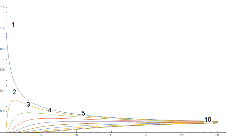
The sum of all solutions is alway '1' - as correctly claimed by @Hans Dolhaine :

Total@mgt // Simplify
(* Out:    1 *)

And all limits seem to be the same - consequently '1/dim', e.g.:

Limit[mgt[[4]], t -> Infinity]
(* Out:   1/10   *)

The dimensionality of this method is quite limited; if you go beyond dim = 10; the calculation time explode. But it seems to show the general behaviour, though.

I suspect it might be related to the boundary conditions...there is a non-conservation at the boundaries because of the interpretation of how to treat the (Mi-1 - Mi) term when i=1. (this can be seen by doing a MatrixForm@update[10, 0.1]). My reading of @MadeleineSutherland's post was that the i-1 term can be discarded, while retaining the i term...but maybe that's not such a physically appropriate idea. Modifying the ends of the matrix to remove these terms should suffice.

To answer the original question: the documentation for NBodySimulation seems to suggest that only position changes are allowed, which would preclude using it for a problem like this.

You could also write this in a functional style (avoiding the use of Do loops) like the following. This is equivalent to @HansDolhaine's first solution above:

    initialState[r_Integer] := {1}~Join~ConstantArray[0, r] 

(*  define a matrix to perform the update step; for large systems, consider using SparseArray*)
(* lump all constants together*)
    update[r_Integer, constants_] := constants*Table[
       (KroneckerDelta[i + 1, j] - KroneckerDelta[i, j]) - (KroneckerDelta[i, j] -KroneckerDelta[i - 1, j]),
     {i, r + 1}, {j, r + 1}]

(*compute a lists of states at each tilmestep*)
results = With[
   {start = initialState[10],
    step = update[10, 0.1],
    timesteps = 20},
   NestList[ (step . # + #) &, start, timesteps]];

ArrayPlot[results] (*watch the magnitization*)

ListLinePlot[Mean /@ results] (*compute properties at each timestep and plot*)