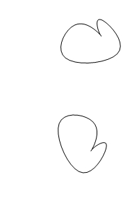
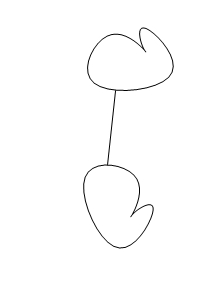
I like the function DistanceTransform. If you are lazy enough, this function provides a lot of "cheap" solutions for complex geometrical problems. For example, one can find the closest pair between two arbitrary set if pixels:
dimensions = {200, 300};
imageXY[{y_, x_}] := {x, dimensions[[2]] + 1 - y};
SetOptions[Graphics,
PlotRange -> {{0, dimensions[[1]]}, {0, dimensions[[2]]}},
ImagePadding -> None, ImageMargins -> 0, PlotRangePadding -> None,
ImageSize -> dimensions, PlotRangeClipping -> True];
pts1 = {{59, 146}, {153, 133}, {128, 76}, {130, 89}, {167, 107}, {116, 17}};
pts2 = ({30, 150} + #) & /@ pts1;
objects = {BSplineCurve[pts1, SplineClosed -> True],
Rotate[BSplineCurve[pts2, SplineClosed -> True], -8 Pi/5]};
Graphics[objects]
Then the closest pair can be found form the distance transform for an individual set:
rasters =
Composition[Binarize, Rasterize[#, ImageSize -> dimensions] &,
Graphics] /@ Table[MapAt[{Opacity[0], #} &, objects, n], {n, 2}];
point1 = imageXY@First@Position[#, RankedMin[Union[Join @@ #], 2]] &[
ImageData[
ImageMultiply[ColorNegate@rasters[[2]],
DistanceTransform@rasters[[1]]]]];
point2 = imageXY@First@Position[#, RankedMin[Union[Join @@ #], 2]] &[
ImageData[
ImageMultiply[ColorNegate@rasters[[1]],
DistanceTransform@rasters[[2]]]]];
Graphics[{objects, Line[{point1, point2}]}]
 Simple labeling
Let's consider the following picture:
dimensions = {350, 500};
nobjects = 8;
radius = 60;
imageXY[{y_, x_}] := {x, dimensions[[2]] + 1 - y};
pts = {{87, 109}, {800/7, 936/7}, {879/7, 1403/7}, {958/7, 1590/
7}, {1429/7, 1721/7}, {1522/7, 2062/7}, {1720/7, 2494/7}, {232,
425}};
densities =
Table[Total[
EuclideanDistance[N@pts[[n]], #] & /@
Nearest[Delete[pts, n], pts[[n]], 5]], {n, nobjects}];
centers = pts[[Reverse@Ordering@densities]];
trajectories = Circle[#, radius] & /@ centers;
objects = Disk[#, radius/5] & /@ centers;
ObjTrj = Transpose[{objects, trajectories}];
Graphics[{ObjTrj, {White, Thread@Text[Range[nobjects], centers]}}]
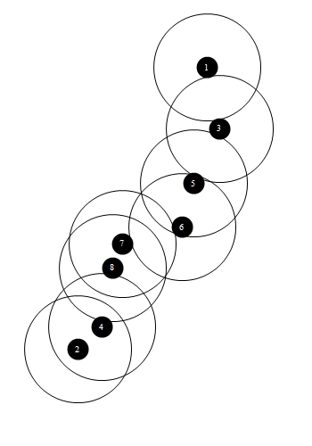
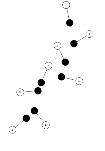
There are discs and circles, below they will be referred as "objects" and "trajectories". Using the same trick as above, one can find a point on a trajectory which is the most distant pixel from all other trajectories. One can use such points as the positions of some labels for the objects. But let me do something smarter. As one can notice I sorted the objects according to their "densities" which are the sum of the distances to the nearest 5 objects. Using this ordering we can make a greedy algorithm for automatic labeling:
SetOptions[Graphics,
PlotRange -> {{0, dimensions[[1]]}, {0, dimensions[[2]]}},
ImagePadding -> None, ImageMargins -> 0, PlotRangePadding -> None,
ImageSize -> dimensions, PlotRangeClipping -> True];
myGraphics[objs_] := Graphics[{blank, objs}];
myRasterize[image_] := Rasterize[image, ImageSize -> (dimensions)];
removeTrajectory[ObjTrj_, n_] := Module[{
distanceMap = DistanceTransform@Binarize@myRasterize@myGraphics@MapAt[{Opacity[0], #} &, ObjTrj, n],
position},
position = imageXY@First@Position[#, Max[#]] &[ImageData[ImageMultiply[trjMasks[[n]], distanceMap]]];
ReplacePart[ObjTrj, n -> {objects[[n]], labelForm[position, centers[[n]], n]}]]
There are three variables should be specified: blank, trjMasks, labelForm
trjMasks = Map[Composition[Binarize, ColorNegate, myRasterize, Graphics], trajectories];
labelForm[pos_, objPos_, n_] := Disk[pos, radius/5];
blank = {};
Their meaning will be clear from applications:
result = Fold[removeTrajectory, ObjTrj, Range[nobjects]];
positions = Composition[First, Last] /@ result;
myGraphics[{objects,
Line /@ Transpose[{centers, positions}],
{White, EdgeForm[Black], Disk[#, radius/5] & /@ positions },
{Black, Thread@Text[Range[nobjects], positions]}}]
Of course, one can use this procedure nested:
result = Fold[removeTrajectory, result, Range[nobjects]];
positions = Composition[First, Last] /@ result;
It convergens very fast:
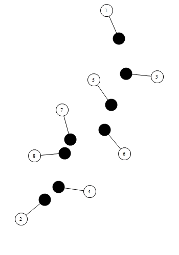
So, you can ask me "why I should use this very slow procedure instead of using an evolution algorithm like that is used for "spring-electrical" embedding for graph drawing?". The reason is that it is much simpler, and more universal, although the result is not optimal in any sense. Firstly, let's change the "blank" variable:
insetSize = 75;
text = Style["This space\n intentionally\n left blank", TextAlignment -> Left];
insetCorner = {113, 639/2};
blank = {Black,
Rectangle[{insetCorner[[1]], insetCorner[[2]] - insetSize}, {insetCorner[[1]] + insetSize, insetCorner[[2]]}]};
The additional black rectangle is autumatically taken into account for optimal labeling:
result = Fold[removeTrajectory, Fold[removeTrajectory, ObjTrj, Range[nobjects]], Range[nobjects]];
positions = Composition[First, Last] /@ result;
myGraphics[{objects,
(Line /@ Transpose[{centers, positions}]), {White, EdgeForm[Black],
Disk[#, radius/5] & /@ positions },
{Black, Thread@Text[Range[nobjects], positions]},
{White, Text[text, insetCorner + {8, -15}, {Left, Top}]}}]
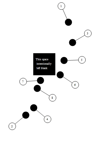
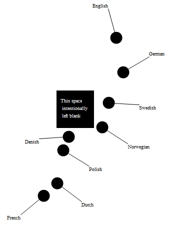
Secondly, let's redefine "labelForm" randering function:
names = {"English", "French", "German", "Dutch", "Swedish",
"Norwegian", "Danish", "Polish"};
labelForm[pos_, objPos_, n_] := {Line[{pos, objPos}],
Text[names[[n]], pos,
Switch[Positive /@ (pos - objPos),
{True, True}, {Left, Bottom},
{True, False}, {Left, Top},
{False, True}, {Right, Bottom},
{False, False}, {Right, Top}]]};
result = Fold[removeTrajectory,
Fold[removeTrajectory, ObjTrj, Range[nobjects]] , Range[nobjects]];
myGraphics[{result, {White,
Text[text, insetCorner + {8, -15}, {Left, Top}]}}]
 Neat example
The art of application of the procedure described above is to choose the nice form of label trajectories. For example, here is a lot of objects (even the boundary of the region is also an object) and linear trajectories:
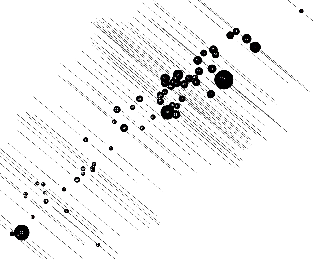
The result of the labeling is the following bubble chart:
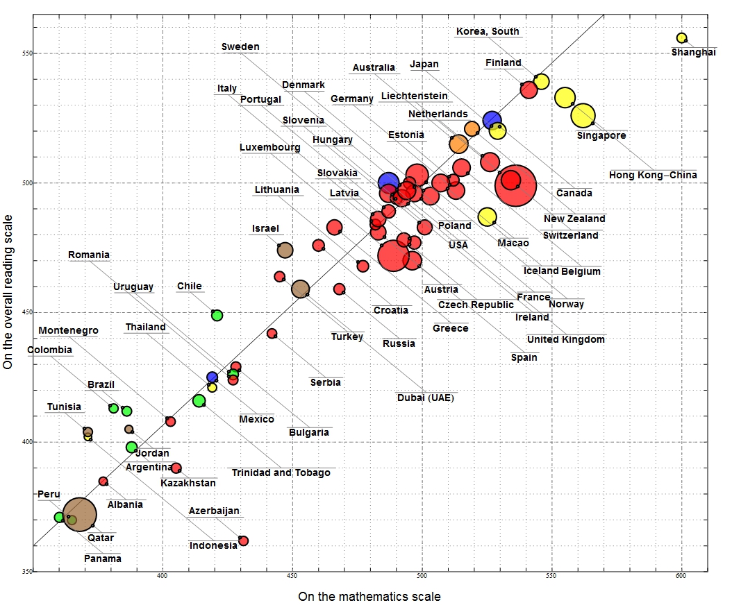
It is the results of
PISA test in 2010. The color of a blob corresponds to some general region (Africa, Europa, North America, Asia etc), the blob size is a linear function of GDP per capita.
 Attachments: