For a true vox file we also need to list colors. This becomes more important when the particular asset has more than two colors. Here is revised export function and an import function to pair with it:
VoxFileFormat[verts_, objname_, SlabSize_, DefaultCols_] := Join[{
   StringJoin["Vox file for ", objname],
   StringJoin[SlabSize, " slab size "],
   "---------------------",
   " x    y    z    c    ",
   "---------------------"},
  Flatten[MapIndexed[Function[{vert},
        Append[vert, #2[[1]] ]] /@ #1 &, verts],
    1] /. {x_, y_, z_, c_} :> StringJoin[
     If[Sign[x] == 1, " ", "-"],
     StringPadRight[ToString[Abs[x]], 4, " "],
     If[Sign[y] == 1, " ", "-"],
     StringPadRight[ToString[Abs[y]], 4, " "],
     If[Sign[z] == 1, " ", "-"],
     StringPadRight[ToString[Abs[z]], 4, " "],
     If[Sign[c] == 1, " ", "-"],
     StringPadRight[ToString[c], 2, " "]
     ], {
   "---------------------",
   " c    R    G    B    ",
   "---------------------"},
  MapIndexed[StringJoin[
     " ", StringPadRight[ToString[#2[[1]]], 4, " "],
     " ", StringPadRight[ToString[#1[[1]]], 4, " "],
     " ", StringPadRight[ToString[#1[[2]]], 4, " "],
     " ", StringPadRight[ToString[#1[[3]]], 4, " "]
     ] &, DefaultCols]
  ]

ToCubes[verts_, cols_] :=  With[
  {colRep = Rule[#[[1]], RGBColor[#[[2 ;; 4]]/255]] & /@ cols},
  {#[[4]] /. colRep, Cuboid[#[[1 ;; 3]]]} & /@ verts]

ImportVox[file_] := With[{lines = StringSplit[Import[file], "\n"]},
  Function[{markers},    ToCubes[ Map[ToExpression, DeleteCases[
       StringSplit[lines[[ markers[[2]] + 1 ;; markers[[3]] - 1  ]],
        " "], "", Infinity], {2}], Map[ToExpression,
      DeleteCases[ StringSplit[lines[[ markers[[4]] + 1 ;; -1  ]], " "], "",
       Infinity], {2}]] ][Flatten[Position[lines, "---------------------"]]]]
I then used the export function to create new files and push to github. Then we can import:
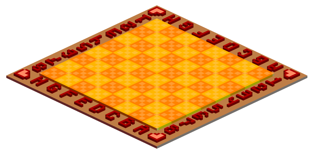
GameBoard =  Graphics3D[{EdgeForm[None],
   ImportVox["~/OpenAssets/WorldChess/TXT/OYChessboardVox.txt"]},
  Boxed -> False, ImageSize -> 1000,
  ViewVertical -> {0, 0, 1}, ViewPoint -> {-100, 100, 75}]
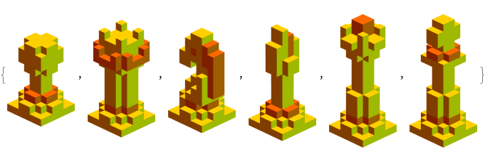
YPieces =  Graphics3D[{EdgeForm[None],
     ImportVox["~/OpenAssets/WorldChess/TXT/Y" <> # <> "Vox.txt"]},
    Boxed -> False, ImageSize -> 100,
    ViewVertical -> {0, 0, 1}, ViewPoint -> {-100, 100, 75}] & /@ ObjNames
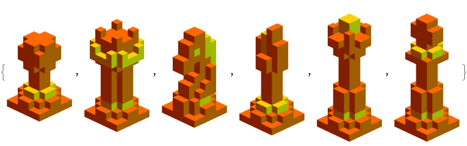
OPieces =  Graphics3D[{EdgeForm[None],
     ImportVox["~/OpenAssets/WorldChess/TXT/O" <> # <> "Vox.txt"]},
    Boxed -> False, ImageSize -> 100, ViewVertical -> {0, 0, 1},
   ViewPoint -> {100, 100, 75}] & /@ ObjNames
Show[ GameBoard,
 YPieces[[1]] /.   Cuboid[{x_, y_, z_}] :>
   Cuboid[{x + 5 + 8 #, y + 13, z + 2}] & /@ Range[0, 7],
 YPieces[[2]] /.   Cuboid[{x_, y_, z_}] :>
     Cuboid[{x + 5 + 8 #, y + 5, z + 2}] & /@ {0, 7},
 YPieces[[3]] /. Cuboid[{x_, y_, z_}] :>
     Cuboid[{y + 5 + 8 #, x + 5, z + 2}] & /@ {1, 6},
 YPieces[[4]] /. Cuboid[{x_, y_, z_}] :>
     Cuboid[{y + 5 + 8 #, x + 5, z + 2}] & /@ {2, 5},
 YPieces[[5]] /. Cuboid[{x_, y_, z_}] :>
     Cuboid[{y + 5 + 8 #, x + 5, z + 2}] & /@ {3},
 YPieces[[6]] /. Cuboid[{x_, y_, z_}] :>
     Cuboid[{y + 5 + 8 #, x + 5, z + 2}] & /@ {4},

 OPieces[[1]] /. Cuboid[{x_, y_, z_}] :>
     Cuboid[{x + 5 + 8 #, y + 13 + 8 5, z + 2}] & /@ Range[0, 7],
 OPieces[[2]] /. Cuboid[{x_, y_, z_}] :>
     Cuboid[{x + 5 + 8 #, -y + 4 + 8 7, z + 2}] & /@ {0, 7},
 OPieces[[3]] /. Cuboid[{x_, y_, z_}] :>
     Cuboid[{y + 5 + 8 #, -x + 4 + 8 7, z + 2}] & /@ {1, 6},
 OPieces[[4]] /. Cuboid[{x_, y_, z_}] :>
     Cuboid[{y + 5 + 8 #, -x + 4 + 8 7, z + 2}] & /@ {2, 5},
 OPieces[[5]] /. Cuboid[{x_, y_, z_}] :>
     Cuboid[{y + 5 + 8 #, -x + 4 + 8 7, z + 2}] & /@ {3},
 OPieces[[6]] /. Cuboid[{x_, y_, z_}] :>
     Cuboid[{y + 5 + 8 #, -x + 4 + 8 7, z + 2}] & /@ {4},
 ViewVertical -> {0, 0, 1}, ViewPoint -> {-100, 100, 75}]
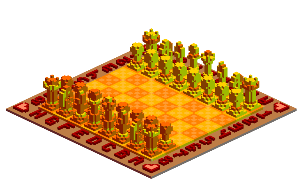
Now if we had a rival player, we could turn this BB into a metaverse by posting and responding, move by move until checkmate is reached, but we might need a few more functions. And while we're at it, here's an article about chess on block chain.


