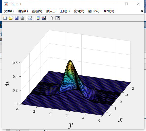
Firstly, the MATLAB programme is
t = 0;
A = 2;
c1 = 1;
c2 = 1;
c = 1/25;
omega = 2;

[xi,eta]=meshgrid(-5:0.1:5,-4:0.1:6);

P = ((2*sinh(xi+omega*t))./(3*cosh(xi+omega*t)))+((5*sinh(xi+omega*t))./(6*cosh(xi+omega*t)).^3)+0.9;
Q = -(sinh(eta))./(cosh(eta));
x = xi-2.5*tanh(xi+omega*t);
y = eta;

Px = -(sech(xi+omega*t)).^2;
Qy = -(sech(eta)).^2;

u = ((A-c1.*c2).*Px.*Qy)./(1+c1.*P+c2.*Q+c.*P.*Q).^2;
view([-45 70]);

surf(x,y,u);
xlabel('x','FontSize',26,'FontName','Times New Roman','FontAngle', 'italic')
ylabel('y','FontSize',26,'FontName','Times New Roman','FontAngle', 'italic')
zlabel('$u$','interpreter','latex','FontSize',24,'FontName','Times New Roman','FontAngle', 'italic')
and it comes
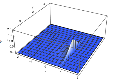
With the same equation, the Mathematica program is
\[Omega] = 2;
A = 2; Subscript[c, 1] = Subscript[c, 2] = 1; Subscript[c, 3] = 1/25;
px = -Sech[\[Xi] + \[Omega] t]^2; p = (2 Sinh[\[Xi] + \[Omega] t])/(
  3 Cosh[\[Xi] + \[Omega] t]) + (5 Sinh[\[Xi] + \[Omega] t])/(
  6 Cosh[\[Xi] + \[Omega] t]^3) + 0.9;
qy = -Sech[\[Eta]]^2; q = -(Sinh[\[Eta]]/Cosh[\[Eta]]);
func[\[Xi]_, \[Eta]_,
   t_] = ((A - Subscript[c, 1] Subscript[c, 2]) px qy)/(1 +
      Subscript[c, 1] p + Subscript[c, 2] q + Subscript[c, 3] p q)^2 //
     Rationalize // Simplify;
xyToXiEta[x_, y_, t_] :=
  NSolve[{x == \[Xi] - 2.5 Tanh[\[Xi] + 2 t],
    y == \[Eta]}, {\[Xi], \[Eta]}, Reals];
With[{t = 0},
 ListPlot3D[
  Flatten[Table[{x, y, func[\[Xi], \[Eta], t]} /.
     xyToXiEta[x, y, t], {x, -2, 2, 0.04}, {y, -1, 5, 0.04}], 2],
  Axes -> True, PlotRange -> {All, All, {0, 2}},
  AxesLabel -> {x, y, z}, ColorFunction -> "TemperatureMap"]]
and it comes
Thanks Gianluca Gorni for providing the Mathematica program.
It is obvious that the MATLAB picture forms like a bridge with empty space under it. However, the Mathematica picture is solid.
How can I improve the Mathematica program to make it like MATLAB's result?
 Attachments:


