WolframAlpha.com
WolframCloud.com
All Sites & Public Resources...
Products & Services
Wolfram|One
Mathematica
Wolfram|Alpha Notebook Edition
Finance Platform
System Modeler
Wolfram Player
Wolfram Engine
WolframScript
Enterprise Private Cloud
Application Server
Enterprise Mathematica
Wolfram|Alpha Appliance
Enterprise Solutions
Corporate Consulting
Technical Consulting
Wolfram|Alpha Business Solutions
Resource System
Data Repository
Neural Net Repository
Function Repository
Wolfram|Alpha
Wolfram|Alpha Pro
Problem Generator
API
Data Drop
Products for Education
Mobile Apps
Wolfram Player
Wolfram Cloud App
Wolfram|Alpha for Mobile
Wolfram|Alpha-Powered Apps
Services
Paid Project Support
Wolfram U
Summer Programs
All Products & Services »
Technologies
Wolfram Language
Revolutionary knowledge-based programming language.
Wolfram Cloud
Central infrastructure for Wolfram's cloud products & services.
Wolfram Science
Technology-enabling science of the computational universe.
Wolfram Notebooks
The preeminent environment for any technical workflows.
Wolfram Engine
Software engine implementing the Wolfram Language.
Wolfram Natural Language Understanding System
Knowledge-based broadly deployed natural language.
Wolfram Data Framework
Semantic framework for real-world data.
Wolfram Universal Deployment System
Instant deployment across cloud, desktop, mobile, and more.
Wolfram Knowledgebase
Curated computable knowledge powering Wolfram|Alpha.
All Technologies »
Solutions
Engineering, R&D
Aerospace & Defense
Chemical Engineering
Control Systems
Electrical Engineering
Image Processing
Industrial Engineering
Mechanical Engineering
Operations Research
More...
Finance, Statistics & Business Analysis
Actuarial Sciences
Bioinformatics
Data Science
Econometrics
Financial Risk Management
Statistics
More...
Education
All Solutions for Education
Trends
Machine Learning
Multiparadigm Data Science
Internet of Things
High-Performance Computing
Hackathons
Software & Web
Software Development
Authoring & Publishing
Interface Development
Web Development
Sciences
Astronomy
Biology
Chemistry
More...
All Solutions »
Learning & Support
Learning
Wolfram Language Documentation
Fast Introduction for Programmers
Wolfram U
Videos & Screencasts
Wolfram Language Introductory Book
Webinars & Training
Summer Programs
Books
Need Help?
Support FAQ
Wolfram Community
Contact Support
Premium Support
Paid Project Support
Technical Consulting
All Learning & Support »
Company
About
Company Background
Wolfram Blog
Events
Contact Us
Work with Us
Careers at Wolfram
Internships
Other Wolfram Language Jobs
Initiatives
Wolfram Foundation
MathWorld
Computer-Based Math
A New Kind of Science
Wolfram Technology for Hackathons
Student Ambassador Program
Wolfram for Startups
Demonstrations Project
Wolfram Innovator Awards
Wolfram + Raspberry Pi
Summer Programs
More...
All Company »
Search
WOLFRAM COMMUNITY
Connect with users of Wolfram technologies to learn, solve problems and share ideas
Join
Sign In
Dashboard
Groups
People
Message Boards
Answer
(
Unmark
)
Mark as an Answer
GROUPS:
Wolfram Science
Mathematics
Algebra
Graphics and Visualization
Graphs and Networks
Wolfram Language
Wolfram Fundamental Physics Project
2
Dmytro Melnichenko
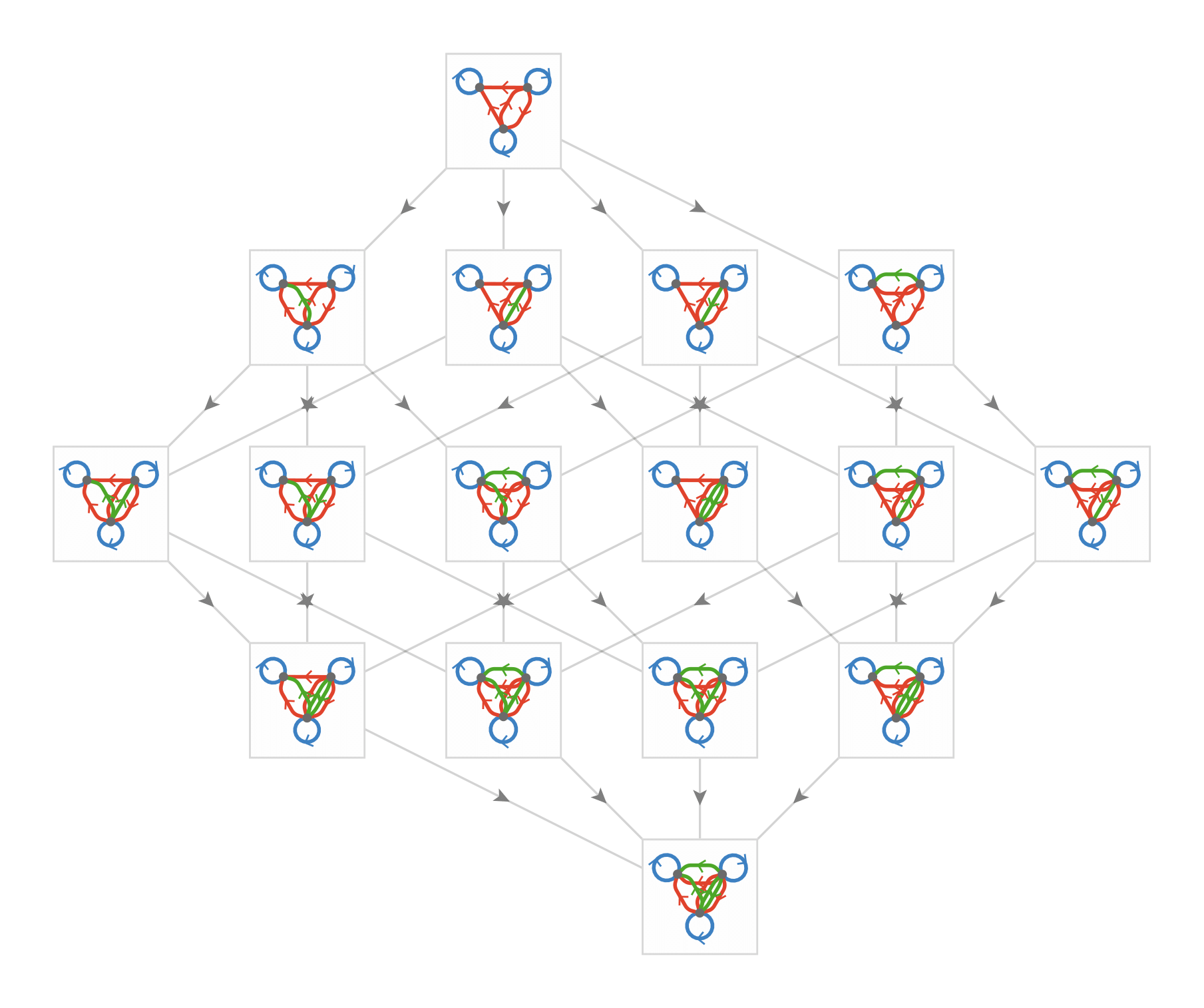
[WWS22] Algebra of graph operators
Dmytro Melnichenko, Physics Student at LMU Munich
Posted
7 months ago
882 Views
|
0 Replies
|
2 Total Likes
Follow this post
|
Algebra of graph operators
by
Dmytro Melnichenko
LMU Munich
The project targets to define product and sum operators represented by the graphs or the hypergraphs. These are used to construct the operator algebra with it. To define the sum and product operations, a suitable matrix representation for the graphs needs to be determined. These operations are later used to construct (anti-) commutators of matrices that describe operators in quantum mechanics and their graphs are studied.
In the scope of the project an ‘edge exclusion hypothesis’ regarding graphs of anti-commuting matrices arose, which claims to find a link between the graphs and their compliments and the anti-commuting properties of matrices.
During the project, multiplication and addition of graphs was represented by the operations on adjacent matrices, which was achieved both using regular definitions and rules for rewrite systems. The latter motivated a new definition of graph - a unigraph, which allowed to achieve confluence for the product operation.
As the rewrite system of the matrix product was only achieved for the adjacency matrices, it would be interesting to see whether/how the same can be implemented for the weighted adjacency matrices. Further, it would be interesting to see, how the ‘edge exclusion hypothesis’ can be generalized for the arbitrary odd dimensional matrices.
Section 1: Sum and Product operations
In the following we will use the weighted graphs, unless stated otherwise. A weighted graph is a graph in which each branch is given a numerical weight. A weighted graph is therefore a special type of labeled graph in which the labels are numbers .
To represent graphs in matrix form, (weighted) adjacency matrices will be used. An adjacency matrix is a square matrix used to represent a finite graph. The elements of the matrix indicate whether pairs of vertices are adjacent or not in the graph. If we consider a matrix B to represent an arbitrary finite graph, the elements of such matrix will be:
1
.
a
n
o
n
-
z
e
r
o
e
l
e
m
e
n
t
B
i
j
t
h
a
t
i
n
d
i
c
a
t
e
s
a
n
e
d
g
e
f
r
o
m
i
t
o
j
2
.
a
z
e
r
o
e
l
e
m
e
n
t
B
i
j
,
i
f
t
h
e
r
e
i
s
n
o
e
d
g
e
f
r
o
m
i
t
o
j
1.1 Sum Rule
I
n
t
h
e
f
o
l
l
o
w
i
n
g
w
e
w
i
l
l
r
e
p
r
e
s
e
n
t
t
h
e
s
u
m
r
u
l
e
o
n
a
n
e
x
a
m
p
l
e
o
f
t
w
o
m
a
t
r
i
c
e
s
A
=
0
2
2
1
a
n
d
B
=
1
1
0
0
a
n
d
t
h
e
r
e
s
u
l
t
i
n
g
m
a
t
r
i
x
C
=
A
+
B
=
1
3
2
1
a
s
g
r
a
p
h
s
.
A
s
a
l
l
t
h
r
e
e
g
r
a
p
h
s
p
o
s
s
e
s
s
t
h
e
s
a
m
e
v
e
r
t
i
c
e
s
,
t
h
e
h
i
g
h
l
i
g
h
t
e
d
e
d
g
e
s
o
f
t
h
e
s
a
m
e
c
o
l
o
r
r
e
p
r
e
s
e
n
t
t
h
e
e
l
e
m
e
n
t
s
o
n
t
h
e
s
a
m
e
p
o
s
i
t
i
o
n
s
f
o
r
e
a
c
h
m
a
t
r
i
x
.
T
h
e
w
e
i
g
h
t
s
o
f
t
h
e
e
d
g
e
s
a
r
e
s
h
o
w
n
t
h
r
o
u
g
h
t
h
e
i
r
t
h
i
c
k
n
e
s
s
.
The graph corresponding to the matrix A looks as follows:
O
u
t
[
]
/
/
M
a
t
r
i
x
F
o
r
m
=
0
2
2
1
O
u
t
[
]
=
And the graph corresponding to the matrix B is:
O
u
t
[
]
/
/
M
a
t
r
i
x
F
o
r
m
=
1
1
0
0
O
u
t
[
]
=
Their sum C is then given as:
O
u
t
[
]
/
/
M
a
t
r
i
x
F
o
r
m
=
1
3
2
1
O
u
t
[
]
=
W
h
e
r
e
t
h
e
l
a
s
t
g
r
a
p
h
i
s
o
b
t
a
i
n
e
d
b
y
c
o
m
b
i
n
i
n
g
t
h
e
h
i
g
h
l
i
g
h
t
e
d
c
o
n
t
r
i
b
u
t
i
o
n
s
o
f
t
h
e
f
i
r
s
t
t
w
o
g
r
a
p
h
s
.
N
o
t
a
b
l
y
,
t
h
e
t
h
i
c
k
n
e
s
s
o
f
t
h
e
o
v
e
r
l
a
p
p
i
n
g
e
d
g
e
s
b
e
t
w
e
e
n
t
h
e
g
r
a
p
h
s
A
a
n
d
B
c
o
n
t
r
i
b
u
t
e
d
t
o
t
h
e
i
n
c
r
e
a
s
e
d
t
h
i
c
k
n
e
s
s
o
f
t
h
e
f
i
n
a
l
g
r
a
p
h
C
.
T
o
s
u
m
m
a
r
i
z
e
:
1.2 Product Rule
S
i
m
i
l
a
r
l
y
t
o
t
h
e
p
r
e
v
i
o
u
s
s
e
c
t
i
o
n
,
w
e
w
i
l
l
r
e
p
r
e
s
e
n
t
t
h
e
p
r
o
d
u
c
t
o
f
t
w
o
m
a
t
r
i
c
e
s
A
=
0
2
2
1
a
n
d
B
=
1
1
0
0
a
n
d
t
h
e
r
e
s
u
l
t
i
n
g
m
a
t
r
i
x
C
=
A
B
=
0
0
2
2
a
s
g
r
a
p
h
s
.
G
e
o
m
e
t
r
i
c
a
l
l
y
o
n
e
c
a
n
v
i
e
w
g
r
a
p
h
m
u
l
t
i
p
l
i
c
a
t
i
o
n
a
s
f
o
l
l
o
w
s
:
S
u
p
p
o
s
e
A
i
s
t
h
e
a
d
j
a
c
e
n
c
y
m
a
t
r
i
x
o
f
g
r
a
p
h
G
1
(
h
i
g
h
l
i
g
h
t
e
d
i
n
g
r
e
e
n
)
a
n
d
B
t
h
e
a
d
j
a
c
e
n
c
y
m
a
t
r
i
x
o
f
g
r
a
p
h
G
2
(
h
i
g
h
l
i
g
h
t
e
d
i
n
b
l
u
e
)
,
w
h
e
r
e
w
e
c
o
n
s
i
d
e
r
b
o
t
h
G
1
a
n
d
G
2
t
o
h
a
v
e
t
h
e
s
a
m
e
v
e
r
t
i
c
e
s
1
,
.
.
.
,
n
.
T
h
e
n
,
(
A
B
)
i
j
i
s
t
h
e
n
u
m
b
e
r
o
f
w
a
y
s
t
o
g
e
t
f
r
o
m
i
t
o
j
b
y
g
o
i
n
g
f
i
r
s
t
a
l
o
n
g
a
n
e
d
g
e
o
f
G
1
a
n
d
t
h
e
n
a
l
o
n
g
a
n
e
d
g
e
o
f
G
2
.
W
e
a
r
e
g
o
i
n
g
t
o
i
l
l
u
s
t
r
a
t
e
t
h
i
s
b
e
l
o
w
.
S
t
a
r
t
i
n
g
w
i
t
h
t
h
e
g
r
a
p
h
r
e
p
r
e
s
e
n
t
a
t
i
o
n
o
f
t
h
e
m
a
t
r
i
x
A
:
O
u
t
[
]
/
/
M
a
t
r
i
x
F
o
r
m
=
0
2
2
1
O
u
t
[
]
=
And the graph representation of the matrix B:
I
n
[
]
:
=
b
m
a
t
=
{
{
1
,
1
}
,
{
∞
,
∞
}
}
;
b
t
h
i
c
k
=
{
1
,
1
}
;
b
c
o
l
o
r
=
{
0
.
7
,
0
.
7
}
;
b
g
r
a
p
h
=
W
e
i
g
h
t
e
d
A
d
j
a
c
e
n
c
y
G
r
a
p
h
[
{
x
,
y
}
,
b
m
a
t
,
V
e
r
t
e
x
L
a
b
e
l
s
-
>
A
u
t
o
m
a
t
i
c
,
E
d
g
e
L
a
b
e
l
s
-
>
A
l
l
,
E
d
g
e
S
t
y
l
e
-
>
T
h
r
e
a
d
[
{
x
-
>
y
,
x
-
>
x
}
-
>
T
h
r
e
a
d
@
{
(
H
u
e
[
#
]
&
/
@
b
c
o
l
o
r
)
,
(
T
h
i
c
k
n
e
s
s
[
#
/
3
0
0
]
&
/
@
b
t
h
i
c
k
)
}
]
,
D
i
r
e
c
t
e
d
E
d
g
e
s
-
>
T
r
u
e
,
E
d
g
e
S
t
y
l
e
-
>
A
r
r
o
w
h
e
a
d
s
[
M
e
d
i
u
m
]
]
;
W
e
i
g
h
t
e
d
A
d
j
a
c
e
n
c
y
M
a
t
r
i
x
[
b
g
r
a
p
h
]
/
/
M
a
t
r
i
x
F
o
r
m
b
g
r
a
p
h
O
u
t
[
]
/
/
M
a
t
r
i
x
F
o
r
m
=
1
1
0
0
O
u
t
[
]
=
First, we compute the matrix AB:
O
u
t
[
]
/
/
M
a
t
r
i
x
F
o
r
m
=
0
0
2
2
O
u
t
[
]
=
The geometric interpretation for each one of four elements of C = AB.
Starting from
(
A
B
)
1
1
: How many ways are there to get from x in
G
1
to x in
G
2
? (The contributing paths are colored in red)
G1:
O
u
t
[
]
=
G2:
O
u
t
[
]
=
Complete path:
I
n
[
]
:
=
As we can see, there is no way of coming to back to x in the graph
G
2
, thus we get
(
A
B
)
1
1
= 0.
(
A
B
)
1
2
: How many ways are there to get from x in
G
1
to y in
G
2
?
G1:
O
u
t
[
]
=
G2:
O
u
t
[
]
=
Complete path:
O
u
t
[
]
=
As there are no self loops in
G
2
, we get
(
A
B
)
1
2
= 0.
(
A
B
)
2
1
: How many ways are there to get from y in
G
1
to x in
G
2
?
G1:
O
u
t
[
]
=
G2:
O
u
t
[
]
=
Complete path:
I
n
[
]
:
=
Remembering that the edges are weighted ( 2 and 1 respectively), we obtain
(
A
B
)
2
1
= 2*1 = 2
(
A
B
)
2
2
: How many ways are there to get from y in
G
1
to y in
G
2
?
G1:
O
u
t
[
]
=
G2:
O
u
t
[
]
=
Complete path:
I
n
[
]
:
=
Thus, we obtain
(
A
B
)
2
2
= 2*1 = 2, which is consistent with the result we obtained above.
1.3 Connection to rewrite systems
I
n
f
o
l
l
o
w
i
n
g
w
e
w
i
l
l
d
e
v
e
l
o
p
a
n
a
l
g
o
r
i
t
h
m
,
w
h
i
c
h
a
p
p
l
i
e
d
t
o
t
h
e
p
a
i
r
o
f
g
r
a
p
h
s
,
p
r
o
d
u
c
e
s
a
n
a
n
a
l
o
g
t
o
t
h
e
g
r
a
p
h
m
u
l
t
i
p
l
i
c
a
t
i
o
n
m
o
t
i
v
a
t
e
d
a
b
o
v
e
.
T
h
i
s
w
i
l
l
b
e
d
o
n
e
i
n
t
w
o
w
a
y
s
:
u
s
i
n
g
t
h
e
u
s
u
a
l
d
i
r
e
c
t
e
d
m
u
l
t
i
g
r
a
p
h
s
a
n
d
t
h
e
u
n
i
g
r
a
p
h
s
.
A
s
a
n
e
x
a
m
p
l
e
,
c
o
n
s
i
d
e
r
t
h
e
g
r
a
p
h
s
r
e
p
r
e
s
e
n
t
e
d
b
y
t
h
e
m
a
t
r
i
c
e
s
A
=
1
1
0
0
,
B
=
0
0
1
1
a
n
d
t
h
e
i
r
p
r
o
d
u
c
t
C
=
A
B
=
1
1
0
0
.
T
h
e
c
o
r
r
e
s
p
o
n
d
i
n
g
g
r
a
p
h
s
a
r
e
:
O
u
t
[
]
=
O
u
t
[
]
=
O
u
t
[
]
=
1.3.1 Directed Multigraphs
In order to keep track of the edges of the given graph pair, we promoted both to the hypergraphs. In doing so, we bind all edges of the first graph A to a point 1 and all the edges of the second graph B we will bind to a point 2. Similarly, the third graph that will result from the manipulations on A and B will be bounded to a point 3. Thus, we can always distinct the three graphs. To implement the graph multiplication using the rewrite system, two rules are defined:
◼
Take an edge from the first graph A and an edge from the second graph B, turn them into an edge in the third graph. Reintroduce the used edges of graphs A, B.
◼
Delete all duplicate edges of the third graph C
O
u
t
[
]
=
,
,
,
Even though, the obtained result does not reach confluence, it still manages to provide the graph multiplication after two generations.
1.3.2 Unigraph
Compared to multigraph, which consists of multiset of pairs, the unigraph consists of sets of pairs. Thus, the problem of confluence is resolved by definition of the set. The elements of matrix representing a unigraph may only contain zeros and ones with the additional rule: 1 + 1 = 1. Application of the unigraph notion to the graph product of A and B results in a graph represented by binary matrix C. While this approach does not preserve weights, the results is confluent.
O
u
t
[
]
=
Section 2: Commutator and Anticommutator
Using the definitions of graph product and graph sum from the previous section, we can now construct the (anti-)commuting matrices and analyze them.
2.1 Commutator
In this section we search for graphs that represent matrices A,B satisfying the following commutation relation:
[A,B] = AB - BA = 0
To simplify the calculations, only symmetric matrices will be considered at the moment. The algorithm of finding the graphs of interest goes as follows:
◼
Pick a random symmetric matrix A
◼
Find its eigenvectors
◼
From the eigenvectors construct another matrix B with random eigenvalues
◼
Visualise the corresponding graphs
The weights of the edges are represented by their opacity, positive weights are colored green and the negative ones are colored purple.
The random commuting matrices and their graphs are given as:
O
u
t
[
]
/
/
M
a
t
r
i
x
F
o
r
m
=
8
.
-
6
.
-
1
.
1
.
-
1
.
-
6
.
8
.
9
.
-
6
.
-
2
.
-
1
.
9
.
-
2
.
1
.
-
3
.
1
.
-
6
.
1
.
-
4
.
2
.
-
1
.
-
2
.
-
3
.
2
.
6
.
O
u
t
[
]
=
O
u
t
[
]
=
Where the maximum difference between two elements is of order of machine precision:
O
u
t
[
]
=
2
.
3
0
9
2
6
×
-
1
4
1
0
An observation can be made at this point: Analogically to how multiple bosons are able to possess the same energy level, so do the edges that can unite the same two vertices in both commuting matrices. This will contrast to how the anti-commuting graphs behave.
2.2 Anticommutator
In this section we search for graphs that represent matrices A, B satisfying the following anti-commutation relation:
{A,B} = AB + BA = 0
2.2.1 Small matrices
F
i
r
s
t
,
w
e
c
a
n
u
s
e
P
a
u
l
i
m
a
t
r
i
c
e
s
a
s
a
n
e
x
a
m
p
l
e
,
w
h
i
c
h
h
a
v
e
t
h
e
p
r
o
p
e
r
t
y
{
σ
j
,
σ
j
}
=
2
δ
i
j
H
e
r
e
,
w
e
w
i
l
l
t
a
k
e
σ
1
=
0
1
1
0
,
σ
2
=
0
-
0
a
n
d
σ
3
=
1
0
0
-
1
.
T
o
r
e
p
r
e
s
e
n
t
e
d
g
e
s
w
i
t
h
n
e
g
a
t
i
v
e
w
i
d
t
h
,
w
e
w
i
l
l
a
l
w
a
y
s
c
o
l
o
r
t
h
e
m
i
n
p
u
r
p
l
e
t
o
m
a
r
k
‘
n
e
g
a
t
i
v
e
t
h
i
c
k
n
e
s
s
’
.
T
h
e
e
d
g
e
s
w
i
t
h
p
o
s
i
t
i
v
e
i
m
a
g
i
n
a
r
y
w
e
i
g
t
h
a
r
e
c
o
l
o
r
e
d
i
n
b
l
u
e
a
n
d
t
h
e
o
n
c
e
s
w
i
t
h
n
e
g
a
t
i
v
e
i
m
a
g
i
n
a
r
y
w
e
i
g
h
t
a
r
e
c
o
l
o
r
e
d
r
e
d
.
T
h
e
c
o
r
r
e
s
p
o
n
d
i
n
g
g
r
a
p
h
f
o
r
σ
1
:
O
u
t
[
]
/
/
M
a
t
r
i
x
F
o
r
m
=
0
.
1
.
1
.
0
.
O
u
t
[
]
=
The corresponding graph for
σ
3
:
O
u
t
[
]
/
/
M
a
t
r
i
x
F
o
r
m
=
1
.
0
.
0
.
-
1
.
O
u
t
[
]
=
And the corresponding anticommutator:
O
u
t
[
]
/
/
M
a
t
r
i
x
F
o
r
m
=
0
0
0
0
Now, let’s compute [
σ
1
,
σ
2
].
The graph of
σ
2
:
O
u
t
[
]
/
/
M
a
t
r
i
x
F
o
r
m
=
0
-
0
O
u
t
[
]
=
And the corresponding anti-commutator:
O
u
t
[
]
/
/
M
a
t
r
i
x
F
o
r
m
=
0
0
0
0
Any graph from above is the complement of the other two (we treat the real and imaginary weights differently). This motivates a hypothesis that two symmetric (self-adjoint) graphs with excluded edges anti-commute, we will call this an ‘edge exclusion hypothesis’.
Conversely, starting from two vertices we can derive Pauli matrices by drawing pairs of graphs with excluded edges. We will develop a more precise formulation of the commuting matrices below. Additionally, using the resulting graphs and the graph corresponding to the unitary matrix, and the product/sum rules from above, we can construct any graph between two vertices.
N
e
x
t
,
w
e
c
a
n
c
o
m
p
u
t
e
t
h
e
a
n
t
i
-
c
o
m
m
u
t
a
t
o
r
s
f
o
r
t
h
e
D
i
r
a
c
m
a
t
r
i
c
e
s
.
T
h
e
l
a
t
t
e
r
o
b
e
y
t
h
e
r
u
l
e
{
μ
γ
,
ν
γ
}
=
2
μ
ν
η
I
4
.
T
h
e
g
r
a
p
h
s
b
e
l
o
w
a
r
e
r
e
p
r
e
s
e
n
t
e
d
b
y
0
γ
,
1
γ
,
2
γ
a
n
d
3
γ
.
0
γ
:
O
u
t
[
]
/
/
M
a
t
r
i
x
F
o
r
m
=
1
.
0
.
0
.
0
.
0
.
1
.
0
.
0
.
0
.
0
.
-
1
.
0
.
0
.
0
.
0
.
-
1
.
O
u
t
[
]
=
1
γ
:
O
u
t
[
]
/
/
M
a
t
r
i
x
F
o
r
m
=
0
.
0
.
0
.
1
.
0
.
0
.
1
.
0
.
0
.
-
1
.
0
.
0
.
-
1
.
0
.
0
.
0
.
O
u
t
[
]
=
2
γ
:
O
u
t
[
]
/
/
M
a
t
r
i
x
F
o
r
m
=
0
0
0
-
0
0
0
0
0
0
-
0
0
0
O
u
t
[
]
=
3
γ
:
O
u
t
[
]
/
/
M
a
t
r
i
x
F
o
r
m
=
0
.
0
.
1
.
0
.
0
.
0
.
0
.
-
1
.
-
1
.
0
.
0
.
0
.
0
.
1
.
0
.
0
.
O
u
t
[
]
=
A
n
d
t
h
e
i
r
c
o
m
m
u
t
a
t
o
r
s
a
r
e
:
0
γ
,
1
γ
}
=
O
u
t
[
]
/
/
M
a
t
r
i
x
F
o
r
m
=
0
0
0
0
0
0
0
0
0
0
0
0
0
0
0
0
0
γ
,
3
γ
=
O
u
t
[
]
/
/
M
a
t
r
i
x
F
o
r
m
=
0
0
0
0
0
0
0
0
0
0
0
0
0
0
0
0
1
γ
,
3
γ
=
O
u
t
[
]
/
/
M
a
t
r
i
x
F
o
r
m
=
0
0
0
0
0
0
0
0
0
0
0
0
0
0
0
0
2
γ
,
3
γ
=
O
u
t
[
]
/
/
M
a
t
r
i
x
F
o
r
m
=
0
0
0
0
0
0
0
0
0
0
0
0
0
0
0
0
Once again, we see that the anti-commuting graphs seem to agree with the ‘edge exclusion hypothesis’.
2.2.2 Generalization for an arbitrary dimension
Now, we can go to an arbitrary dimension, by considering higher-dimensional gamma matrices. We farther restrict ourselves to the discussion of even dimensions d = 2k, k in {1, 2, 3, ...} and towards the first and the second to last and the last gamma matrix
Γ
0
,
Γ
d
and
Γ
d
+
1
respectively.
The algorithm for constructing these matrices is recursive and the new matrices
Γ
a
, (a = 0, ..., d+1) given by:
◼
Γ
0
=
γ
0
σ
3
◼
Γ
d
= I
(
σ
1
)
◼
Γ
d
+
1
= I
(
σ
2
)
Where
γ
0
comes from the previous system with
γ
b
, (b = 0, ..., d-1).
As an example, we may consider 16x16 gamma matrices.
Γ
0
:
O
u
t
[
]
=
Γ
d
:
O
u
t
[
]
=
Γ
d
+
1
:
O
u
t
[
]
=
And the corresponding matrices indeed commute up to machine precision:
{
Γ
0
,
Γ
d
+
1
}=
O
u
t
[
]
=
0
.
{
Γ
d
,
Γ
d
+
1
}=
O
u
t
[
]
=
0
.
W
h
e
r
e
w
e
o
n
c
e
a
g
a
i
n
c
o
n
c
l
u
d
e
t
h
e
‘
e
d
g
e
e
x
c
l
u
s
i
o
n
h
y
p
o
t
h
e
s
i
s
’
.
I
t
c
a
n
b
e
s
h
o
w
n
t
h
a
t
f
o
r
t
h
e
g
r
a
p
h
s
o
f
e
v
e
n
d
i
m
e
n
s
i
o
n
w
i
t
h
r
e
a
l
w
e
i
g
h
t
s
t
o
a
n
t
i
-
c
o
m
m
u
t
e
,
t
h
e
y
m
u
s
t
h
a
v
e
t
h
e
f
o
l
l
o
w
i
n
g
f
o
r
m
A
=
a
⋯
0
⋮
⋱
⋮
0
⋯
-
a
a
n
d
t
h
e
o
t
h
e
r
m
a
t
r
i
c
e
s
B
i
a
r
e
f
i
l
l
e
d
w
i
t
h
n
o
n
-
d
i
a
g
o
n
a
l
e
l
e
m
e
n
t
s
.
2.2.3 Edge exclusion hypothesis
I
n
o
r
d
e
r
t
o
s
t
u
d
y
t
h
e
e
d
g
e
e
x
c
l
u
s
i
o
n
h
y
p
o
t
h
e
s
i
s
f
u
r
t
h
e
r
,
w
e
h
a
v
e
d
e
v
i
s
e
d
a
n
o
t
h
e
r
t
e
s
t
.
F
o
r
t
h
a
t
w
e
t
a
k
e
a
n
a
b
s
o
l
u
t
e
v
a
l
u
e
o
f
a
n
a
d
j
a
c
e
n
c
y
m
a
t
r
i
x
r
e
p
r
e
s
e
n
t
i
n
g
a
c
e
r
t
a
i
n
g
r
a
p
h
a
n
d
c
o
m
p
u
t
e
i
t
s
c
o
m
p
l
e
m
e
n
t
.
T
h
e
l
a
t
t
e
r
i
s
d
e
f
i
n
e
d
t
o
e
x
c
h
a
n
g
e
t
h
e
z
e
r
o
s
w
i
t
h
o
n
e
s
a
n
d
v
i
c
e
v
e
r
s
a
f
o
r
e
a
c
h
e
l
e
m
e
n
t
o
f
t
h
e
m
a
t
r
i
x
.
T
h
i
s
i
s
d
e
m
o
n
s
t
r
a
t
e
d
o
n
a
n
e
x
a
m
p
l
e
o
f
t
h
e
P
a
u
l
i
m
a
t
r
i
x
σ
1
=
0
1
1
0
b
e
l
o
w
:
I - abs(
σ
1
) =
O
u
t
[
]
/
/
M
a
t
r
i
x
F
o
r
m
=
1
0
0
1
N
e
x
t
s
t
e
p
i
s
t
o
c
o
m
p
u
t
e
t
h
e
e
l
e
m
e
n
t
w
i
s
e
i
n
t
e
r
s
e
c
t
i
o
n
b
e
t
w
e
e
n
t
h
e
c
o
m
p
l
i
m
e
n
t
o
f
t
h
e
g
i
v
e
n
m
a
t
r
i
x
a
n
d
t
h
e
a
b
s
o
l
u
t
e
v
a
l
u
e
o
f
a
c
o
m
m
u
t
i
n
g
m
a
t
r
i
x
.
T
h
e
i
n
t
e
r
s
e
c
t
i
o
n
i
s
d
e
f
i
n
e
d
t
o
g
i
v
e
o
n
e
,
i
f
b
o
t
h
m
a
t
r
i
x
e
l
e
m
e
n
t
s
a
r
e
o
n
e
a
n
d
i
s
z
e
r
o
o
t
h
e
r
w
i
s
e
.
F
o
r
e
x
a
m
p
l
e
,
t
h
e
i
n
t
e
r
s
e
c
t
i
o
n
o
f
t
h
e
c
o
m
p
l
i
m
e
n
t
o
f
σ
1
w
i
t
h
t
h
e
a
b
s
o
l
u
t
e
v
a
l
u
e
o
f
σ
3
=
1
0
0
-
1
:
O
u
t
[
]
/
/
M
a
t
r
i
x
F
o
r
m
=
1
0
0
1
Finally, we count ones and divide by the matrix dimension. For the example above we get:
O
u
t
[
]
=
1
Doing the same operation for the Dirac matrices and higher dimensional matrices, we obtain a plot:
O
u
t
[
]
=
As the number of intersections per dimension does not grow for the bigger matrices, we may indeed conclude, that there is a pattern present. Thus, the plot is in the agreement with an assumption of the ‘edge exclusion hypothesis’ in higher-order gamma matrices.
Concluding remarks
The algebra of graph operators has proven to be an interesting topic with a large number of undiscovered properties. In scope of this project, we have shown the multiple ways to define a graph product, especially the definition with regards to unigraph seems to have a lot of potential.
Using the operations of addition and multiplication, we have found a way to construct (anti-)commuting graphs. In case of the anti-commutation, a farther insight has been provided - two graphs that have excluded edges anti-commute, this has been called an ‘edge exclusion hypothesis’, as it is similar to the Pauli exclusion principle for the fermions.
In the future it would be meaningful to investigate the project further for the following points still need to be addressed:
◼
Isomorphism of local subgraphs of the the graph product multiway system
◼
Generalization of the graph product using the rewrite system to the weighted graphs, retaining the confluence
◼
Search for topological properties in (anti-)commuting graphs
◼
Proof and further generalization of the edge exclusion hypothesis
◼
Discussion of odd-dimensional (anti-)commuting graphs
Keywords
◼
Adjacency Matrix
◼
Graph Product
◼
Unigraph
◼
Commuting Graphs
◼
Anti-commuting Graphs
◼
Edge exclusion hypothesis
Acknowledgment
I would like to sincerely thank my mentors, Xerxes Arsiwalla and Jon Lederman, for their invaluable input and support. Also, I can’t over-appreciate the help of Tali Beynon, who explained a lot of graph theory and wrote a function for the discussion of unigraphs.
My gratitude goes to Steven Wolfram, who helped define my project and made valuable comments during the Mid-Course corrections.
References
◼
Adjacency matrix:
https://en.wikipedia.org/wiki/Adjacency_matrix
◼
Adjacency:
https://quivergeometry.net/adjacency/#matrix_powers _and _walks
◼
Multisets:
https://quivergeometry.net/multisets/
◼
Higher-order Gamma Matrices:
https://en.wikipedia.org/wiki/Higher-dimensional_gamma _matrices
◼
Graph Product:
https://math.stackexchange.com/questions/114334/product-of-adjacency-matrices
Attachments:
Graph Operators ...pdf
POSTED BY:
Dmytro Melnichenko
Reply
|
Flag
Reply to this discussion
in reply to
Add Notebook
Community posts can be styled and formatted using the
Markdown syntax
.
Tag limit exceeded
Note: Only the first five people you tag will receive an email notification; the other tagged names will appear as links to their profiles.
Publish anyway
Cancel
Reply Preview
Attachments
Remove
Add a file to this post
Follow this discussion
or
Discard
Group Abstract
Be respectful. Review our
Community Guidelines
to understand your role and responsibilities.
Community Terms of Use
Feedback
Enable JavaScript to interact with content and submit forms on Wolfram websites.
Learn how »