WOLFRAM MATERIALS for the ARTICLE:
Mohammad, M.; Trounev, A.; Alshbool, M.
A Novel Numerical Method for Solving Fractional Diffusion-Wave and Nonlinear Fredholm and Volterra Integral Equations with Zero Absolute Error.
Axioms 2021, 10, 165.
https://doi.org/10.3390/axioms10030165
Abstract
The new numerical method for linear and nonlinear Poisson's equations in 2D and 3D is proposed. The method is based on the Bernoulli, Chebyshev or Euler wavelets and the Newton's iterative method. Several examples with known exact solutions have been solved with zero absolute error.
Introduction
Recently we have reported the higher precision numerical solution with zero absolute error for nonlinear Volterra and Fredholm integral equation and for the linear and nonlinear fractional diffusion wave equation . We used the Euler wavelets collocation method to solve the linear and nonlinear mathematical problems. Since even for nonlinear problems we got zero absolute error, we have suggested that there is some numerical phenomenon of error cancellation. In this paper we proposed the new numerical method to solve linear and nonlinear Poisson's equations in 2D and in 3D. The effective numerical method for the Poisson's equation is very important in many applications in physics, fluid dynamics, structural mechanics and others. In general case nonlinear Poisson's equation can be written as follows
$$ \nabla^2 u=F(\mathbf{r},u,\nabla u) $$ where $F$ is some function, and $\mathbf{r}=(x,y,z)$. In this research we will consider Poisson's equation on the unit rectangle $0\le x\le 1,0\le y\le 1$, and in the unit cube $0\le x\le 1,0\le y\le 1, 0\le z\le 1$ with Dirichlet type boundary conditions.
Numerical algorithm for 2D problems
The numerical method described in our paper is based on Euler wavelets which involve polynomials $E_1(x), E_2(x)$ only. Her we extend wavelets truncated system with more degrees of $E_n, n=1, 2, 3, ...$. We define Euler polynomials $E_n(x)$ in general case as
$$\frac{2 e^{x t}}{e^t+1}=\sum_0^\infty E_n(x)\frac{t^n}{n!}$$
We can generate family of Euler wavelets using Euler polynomials as follows
$$ \psi(k,n,m,t)=2^{k/2} \sqrt{2/\pi} E_m(2^k t - 2 n + 1), \frac{n-1}{2^{k-1}} \le t < \frac{n}{2^{k-1}}$$ and $ \psi(k,n,m,t) = 0$, otherwise. Let define vector with fixed length $N=M 2^{k-1}$ and integrals of it in the form
$$\Psi_{k M}(t)=(\psi(k,1,0,t),...,\psi(k,2^{k-1},M-1,t))$$
$$ I_1(t)=\int_0^t\Psi_{k M}(t)d t$$
$$ I_2(t)=\int_0^t I_1(t)d t$$
With these definitions we can define solution of Poisson's equation by integrating two equations
$$ u_{xx}=\Psi_{k M}^T(x).U_1.\Psi_{k M}(y) $$
$$ u_{yy}=\Psi_{k M}^T(y).U_2.\Psi_{k M}(x) $$ where $U_1,U_2$ are matrices by $N\times N$ should be determined with using collocation points. Integrating equation for $u_{xx}, u_{yy}$ step by step we have
$$ u_{x}=I_1^T(x).U_1.\Psi_{kM}(y)+G_1.\Psi_{kM}(y) $$
$$ u_1(x,y)=I_2^T(x).U_1.\Psi_{kM}(y)+x G_1.\Psi_{kM}(y)+u_b(0,y) $$
$$ u_{y}=I_1^T(y).U_2.\Psi_{kM}(x)+G_2.\Psi_{kM}(x) $$
$$ u_2(x,y)=I_2^T(y).U_2.\Psi_{kM}(x)+y G_2.\Psi_{kM}(x)+u_b(x,0) $$
Here $G_1,G_2$ are some vectors of length $N$ to be computed. Finally we define $N$ collocation points and compute equations in collocation points, we have $$ u_{xx}(x_i,y_j)+u_{yy}(x_i,y_j)=F(x_i,y_j,u(x_i,y_j),u_x(x_i,y_j),u_y(x_i,y_j)) $$ $$ u_1(x_i,y_j)=u_2(x_i,y_j) $$ $$ u_1(1,y_j)=u_b(1,y_j) $$ $$ u_2(x_i,1)=u_b(x_i,1)$$ $ i,j=1,2,...,N$,
$$ \Delta x=1/N, s_0=0, s_i=s_{i-1}+\Delta x, i=1,2,..,N, x_i=y_i=\frac{1}{2}(s_{i-1}+s_{i}), i=1,2,...,N $$
The system of nonlinear algebraic equations shown above can be solved by the Newton's iterative method. Let consider Poisson's equation on the unit square solved by Lepik in the paper with collocation method based on Haar wavelets $$ u_{xx}+u_{zz}=6 (1 - x) x^3 (1 - z) z - 6 (1 - x) x^3 z^2 + 6 (1 - x) x (1 - z) z^3 - 6 x^2 (1 - z) z^3 $$ Exact solution of this equation with homogeneous boundary condition $u(x,z)=0$ is $$ u=x^3 z^3 (1 - x) (1 - z) $$ The maximal absolute error of numerical solution computed with the Lepik's method is given by $\delta = 9.4\times 10^{-5}, 2.4\times 10^{- 5}, 6.0\times 10^{-6}$ for number of collocation points $N=8, 16, 32$ consequently. With our method we can solve this example with zero absolute error for $N=6, 8, 12, 16$ - see Figure 1. 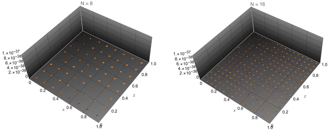 Code to generate solution with zero absolute error for this case is given by
 Q[x_, z_] :=
 6 (1 - x) x^3 (1 - z) z - 6 (1 - x) x^3 z^2 +
  6 (1 - x) x (1 - z) z^3 - 6 x^2 (1 - z) z^3;
ue[x_, z_] := x^3 z^3 (1 - x) (1 - z);

UE[m_, t_] := EulerE[m, t]
psi[k_, n_, m_, t_] :=
 Piecewise[{{2^(k/2) Sqrt[2/Pi] UE[m, 2^k t - 2 n + 1], (n - 1)/
      2^(k - 1) <= t < n/2^(k - 1)}, {0, True}}]
PsiE[k_, M_, t_] :=
 Flatten[Table[psi[k, n, m, t], {n, 1, 2^(k - 1)}, {m, 0, M - 1}]]
k0 = 2; M0 = 3; With[{k = k0, M = M0},
 var1 = Flatten[Table[c[n, m], {n, 1, 2^(k - 1)}, {m, 0, M - 1}]]];
nn = Length[var1]
dx = 1/(nn);  xl = Table[ l*dx, {l, 0, nn}]; zcol =
 xcol = Table[(xl[[l - 1]] + xl[[l]])/2, {l, 2, nn + 1}]; Psijk =
 With[{k = k0, M = M0}, PsiE[k, M, t1]]; Int1 =
 With[{k = k0, M = M0}, Integrate[PsiE[k, M, t1], t1]];
Int2 = Integrate[Int1, t1]; Psi[y_] := Psijk /. t1 -> y;
int1[y_] := Int1 /. t1 -> y; int2[y_] := Int2 /. t1 -> y;
M = nn;

U1 = Array[a, {M, M}]; U2 = Array[b, {M, M}]; G1 =
 Array[g11, {M}]; G2 = Array[g12, {M}];


u1[x_, z_] := int2[x] . U1 . Psi[z] + x G1 . Psi[z] + ue[0, z];
u2[x_, z_] := Psi[x] . U2 . int2[z] + z G2 . Psi[x] + ue[x, 0];
uz[x_, z_] := Psi[x] . U2 . int1[z] + G2 . int1[z];
ux[x_, z_] := int1[x] . U1 . Psi[z] + G1 . Psi[z];
uxx[x_, z_] := Psi[x] . U1 . Psi[z];
uzz[x_, z_] := Psi[x] . U2 . Psi[z];


eq = Join[
  Flatten[Table[(uxx[xcol[[i]], zcol[[j]]] +
        uzz[xcol[[i]], zcol[[j]]]) - Q[xcol[[i]], zcol[[j]]] == 0, {i,
      M}, {j, M}]],
  Flatten[Table[
    u1[xcol[[i]], zcol[[j]]] - u2[xcol[[i]], zcol[[j]]] == 0, {i,
     M}, {j, M}]],
  Flatten[Table[u1[1, zcol[[j]]] - ue[1, zcol[[j]]] == 0, {j, M}]],
  Flatten[Table[
    u2[xcol[[j]], 1] - ue[xcol[[j]], 1] == 0, {j, M}]]]; var =
 Join[Flatten[U1], Flatten[U2], G1, G2];
sol = FindRoot[eq, Table[{var[[i]], 1/10}, {i, Length[var]}],
   MaxIterations -> 1000, WorkingPrecision -> 100];

lst2 = Flatten[
   Table[{x, t, Abs[ue[x, t] - u1[x, t] /. sol]}, {x, xcol}, {t,
     zcol}], 1];

ListPointPlot3D[lst2, PlotTheme -> "Marketing",
 AxesLabel -> {x, y, ""}, PlotLabel -> Row[{"N = ", nn}],
 PlotStyle -> Orange, PlotRange -> {{0, 1}, {0, 1}, {0, 10^-37}}]
Note, that we put limit on the plot $10^{-37}$ while if we evaluate lst2 then we have zero absolute error in every collocation point
Out[]= {{1/12, 1/12, 0.*10^-103}, {1/12, 1/4, 0.*10^-104}, {1/12, 5/
  12, 0.*10^-104}, {1/12, 7/12, 0.*10^-103}, {1/12, 3/4,
  0.*10^-104}, {1/12, 11/12, 0.*10^-104}, {1/4, 1/12, 0.*10^-103}, {1/
  4, 1/4, 0.*10^-103}, {1/4, 5/12, 0.*10^-103}, {1/4, 7/12,
  0.*10^-102}, {1/4, 3/4, 0.*10^-103}, {1/4, 11/12, 0.*10^-103}, {5/
  12, 1/12, 0.*10^-102}, {5/12, 1/4, 0.*10^-103}, {5/12, 5/12,
  0.*10^-103}, {5/12, 7/12, 0.*10^-102}, {5/12, 3/4, 0.*10^-102}, {5/
  12, 11/12, 0.*10^-102}, {7/12, 1/12, 0.*10^-102}, {7/12, 1/4,
  0.*10^-102}, {7/12, 5/12, 0.*10^-102}, {7/12, 7/12, 0.*10^-102}, {7/
  12, 3/4, 0.*10^-102}, {7/12, 11/12, 0.*10^-102}, {3/4, 1/12,
  0.*10^-102}, {3/4, 1/4, 0.*10^-102}, {3/4, 5/12, 0.*10^-102}, {3/4,
  7/12, 0.*10^-101}, {3/4, 3/4, 0.*10^-102}, {3/4, 11/12,
  0.*10^-102}, {11/12, 1/12, 0.*10^-101}, {11/12, 1/4,
  0.*10^-102}, {11/12, 5/12, 0.*10^-102}, {11/12, 7/12,
  0.*10^-101}, {11/12, 3/4, 0.*10^-101}, {11/12, 11/12, 0.*10^-101}}
Several numerical examples and extension this method to the 3D are described in the paper attached.
 Attachments:


