Just to put into words what is going on.
You defined the vector field in VectorPlot to be {(x-y)/(x+y), x}.
The vector field should be {1, (x-y)/(x+y)}.
General remark: A vector field of the form
$(v_x, v_y)$ represents the system of differential equations
$dx/dt = v_x$,
$dy/dt = v_y$.
Thus a vector field of the form
$(1, f(x, y))$ represents the system
$dx/dt = 1$,
$dy/dt = f(x, y))$. Since
$dy/dx = \big(dy/dt\big) \big/ \big(dx/dt\big)$, this system is equivalent to
$dy/dx = f(x,y)$.
Gratuitous remarks:
The integration parameter shows up as E^(2 C[1]), which can be negative if C[1] is complex. This is inconvenient, perhaps. We can replace C[1] -> Log[c1]/2 to get simply c1 as a parameter, which now give negative term inside Sqrt[] whenever c1 is negative.
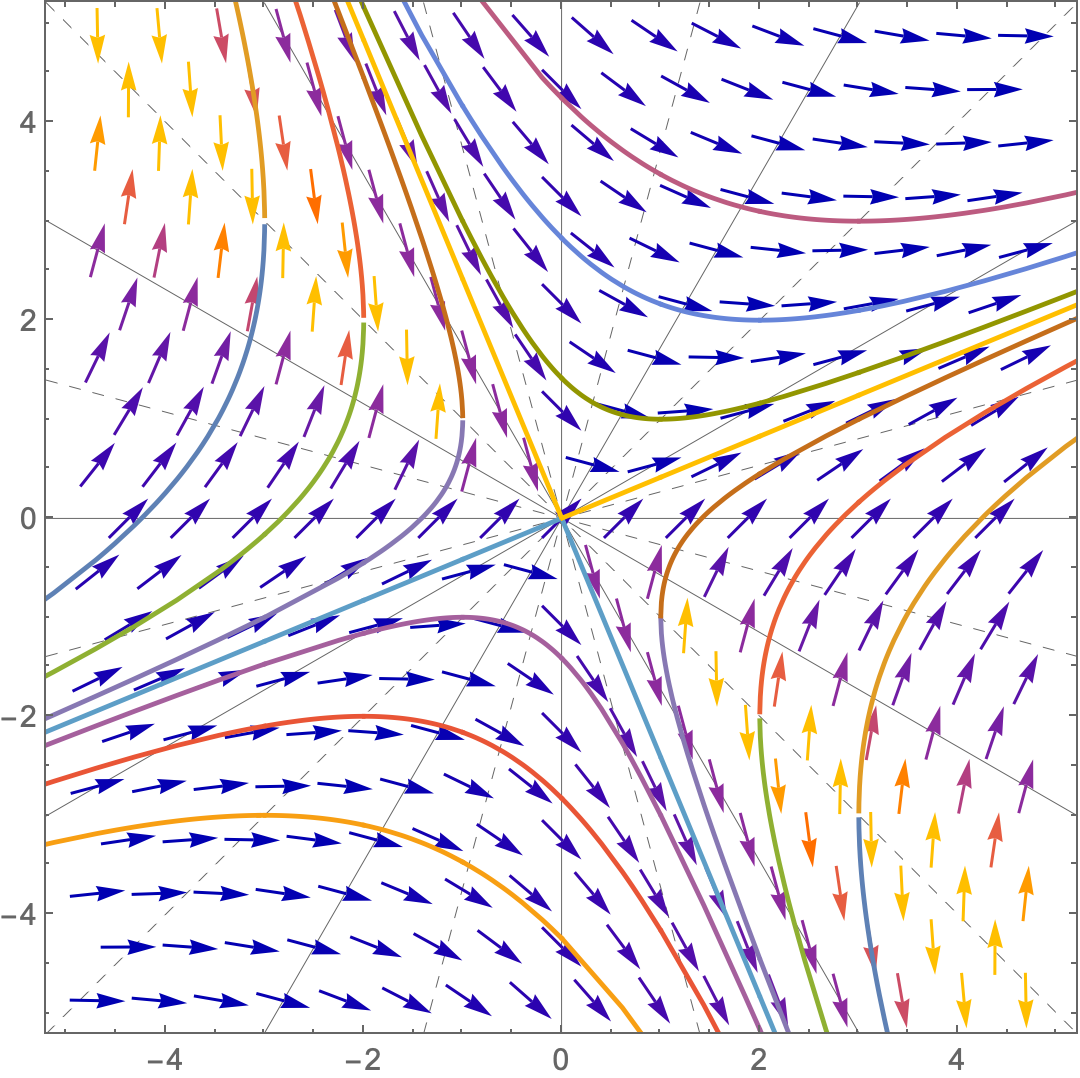
A characteristic of homogeneous DEs is that the integral curves cross a radial line at the same angle. Since in recent versions of WL in VectorPlot, many vectors lie on radial lines at angles of 0º, 30º, 60º, etc., this is easy to show.
solhomo2 = solhomo /. C[1] -> Log[c1]/2  (* put parameter in a convenient form *)
(*  {{y[x] -> -x - Sqrt[c1 + 2 x^2]}, {y[x] -> -x + Sqrt[c1 + 2 x^2]}}  *)

funcionesh = Flatten@Table[y[x] /. solhomo2,
  {c1, 2 Abs[#] # &@Range[-3, 3]}]; (* c1 = ±2 times squares *)
Show[
  VectorPlot[{1, (x - y)/(x + y)}, {x, -5, 5}, {y, -5, 5},
    (*Axes->True,AxesStyle->Black,Axes->Black,*)
    Prolog -> { (* omit axes, add radial lines *)
      Thin, Black,
      Table[
        InfiniteLine[{0, 0}, {Cos[t], Sin[t]}], {t, 0, 5 Pi/6, Pi/6}],
      Dashed,
      Table[
        InfiniteLine[{0, 0}, {Cos[t], Sin[t]}], {t, Pi/12, Pi, Pi/6}]}
   ],
  Plot[funcionesh, {x, -10, 10}]
]