WOLFRAM MATERIALS for the FUNCTION:
Bradley Klee (2022). FindExactCover: Find row subsets of an input binary matrix that sum to 1 in each column. Wolfram Function Repository.
https://resources.wolframcloud.com/FunctionRepository/resources/FindExactCover/
Recently we've published FindExactCover through Wolfram Function Repository. This is a flexible resource with three distinct methods for solving exact cover problems. One explanation why we ended up needing so many methods is the well-known slipperiness of non-polynomial-time (NP) problems--They can easily change from one form to another. There are a variety of different algorithms whose practical efficiency at solving one particular problem depends on what input form allows the most natural encoding of the details, so it's always necessary to have a few different approaches ready. The purpose of this memo is to explain one use case which is well targeted by Knuth's Dancing Links X algorithm. And yes, it's also another one about making artsy snowflake plots for this winter season.
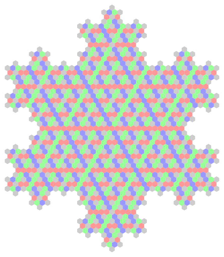
The starting point for this exploration is a speculative post we made last year about creating symmetric shapes with fractal boundaries suggestive of snowflakes. Let us take one of the better patterns we found from the "whole-hex" substitution system:
symStar = ReIm[Exp[I 2 Pi #/3]] & /@ Range[0, 2];

ToCanonical[vec_] := Subtract[vec, Floor[Divide[vec . {1, 1, 1}, 3]]]

InflateRep = {T[x_, v_] :>
    With[{InfM = Times[IdentityMatrix[3], 3]}, Prepend[
      Join[
       T[ToCanonical[InfM . x + IdentityMatrix[3][[#]]], #] & /@
        Range[3],
       T[ToCanonical[InfM . x - IdentityMatrix[3][[#]]], #] & /@
        Range[3],
       T[ToCanonical[
           InfM . x + IdentityMatrix[3][[#]] -
            IdentityMatrix[3][[# /. {1 -> 2, 2 -> 3, 3 -> 1}]]],
          0] & /@ Range[3],
       T[ToCanonical[
           InfM . x - IdentityMatrix[3][[#]] +
            IdentityMatrix[3][[# /. {1 -> 2, 2 -> 3, 3 -> 1}]]],
          0] & /@ Range[3]], T[ToCanonical[InfM . x], v]]]};

Depict[v_, c_, star_ : symStar] := {c /. {
     1 -> Lighter[#, .6] &@Red,
     2 -> Lighter[#, .6] &@Blue,
     3 -> Lighter[#, .6] &@Green
     , 0 -> Lighter[Gray, .6], 0 -> White},
   Polygon[CirclePoints[v . star,
     {1/Sqrt[3], Pi/6}, 6]]};

Graphics[
 Nest[Union[Flatten[# /. InflateRep]] &, T[{0, 0, 0}, 1], 3] /.
  T -> Depict]
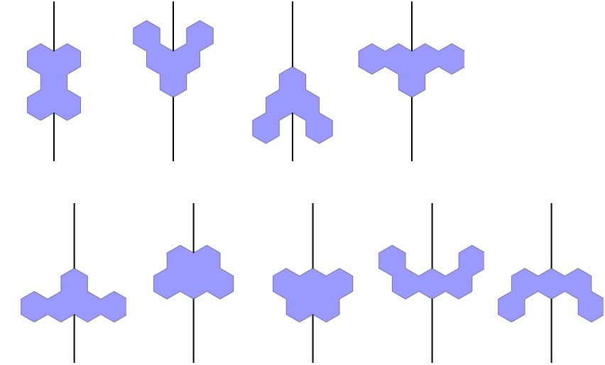
Rather than trying to replicate the pattern with a cellular automata, we will leave the pattern as is, and pave it over with pentahexes. The pentahexes are a special set of polyhexes, which are generated recursively from a single hexagon by joining on edge as follows:
IterateAddHex[state_
  ] := Union[Map[Function[ptlist,
    First@Union[Union /@ Outer[
          Expand[RotationMatrix[Pi/3 #1] . #2] &,
          Range[6], #, 1],
        Union /@ Outer[
          Expand[RotationMatrix[Pi/3 #1] . Times[#2, {1, -1}]] &,
          Range[6], #, 1]] &[# - Mean[ptlist] & /@ ptlist]],
   If[Not[MemberQ[state, #]], Append[state, #],
      Nothing] & /@ Catenate[
     Outer[Expand@*Plus, state, CirclePoints[6], 1]]]]

PolyhexPrimitive[vertices_] := With[{edges = Map[
     UndirectedEdge @@ Sort[#] & /@ Partition[
        Simplify@CirclePoints[#, {1/Sqrt[3], Pi/6},
          6], 2, 1, 1] &, vertices]},
  Polygon[First /@ First[FindCycle[
      Graph[First /@ Select[Gather[Catenate[edges]],
         Length[#] == 1 &]]
      ]]]]

With[{g1 = NestGraph[IterateAddHex, {{{0, 0}}}, 4,
    EdgeStyle -> Gray,
    VertexShapeFunction -> (With[
        {phex = PolyhexPrimitive[#2]},
        Inset[Graphics[{Lighter[Blue, .7], EdgeForm[Thin], phex},
          PlotRange -> {
            MinMax[phex[[1, All, 1]]] + {-0.1, 0.1},
            MinMax[phex[[1, All, 2]]] + {-0.1, 0.1}},
          ImageSize -> {
            20 MinMax[phex[[1, All, 1]]] + {-0.1, 0.1},
            20 MinMax[phex[[1, All, 2]]] + {-0.1, 0.1}}
          ], #1, Automatic]] &),
    PerformanceGoal -> "Quality", AspectRatio -> 1/2,
    GraphLayout -> "LayeredDigraphEmbedding"]},
 Graph[g1,
  ImageSize -> 620,
  PerformanceGoal -> "Quality",
  VertexCoordinates -> MapThread[Rule, {VertexList[g1],
     ReplacePart[
      GraphEmbedding[g1],
      MapIndexed[#[[1]] -> (#[[2]] - {Mod[#2[[1]] + 1, 2]/4,
            Mod[#2[[1]] + 1, 2]/1.5 + 2 Mod[#2[[1]], 2]}) &,
       SortBy[# -> GraphEmbedding[g1][[#]] & /@
         Catenate[Position[Length /@ VertexList[g1], 5]],
        First[Last[#]] &
        ]]]}]]
 ]
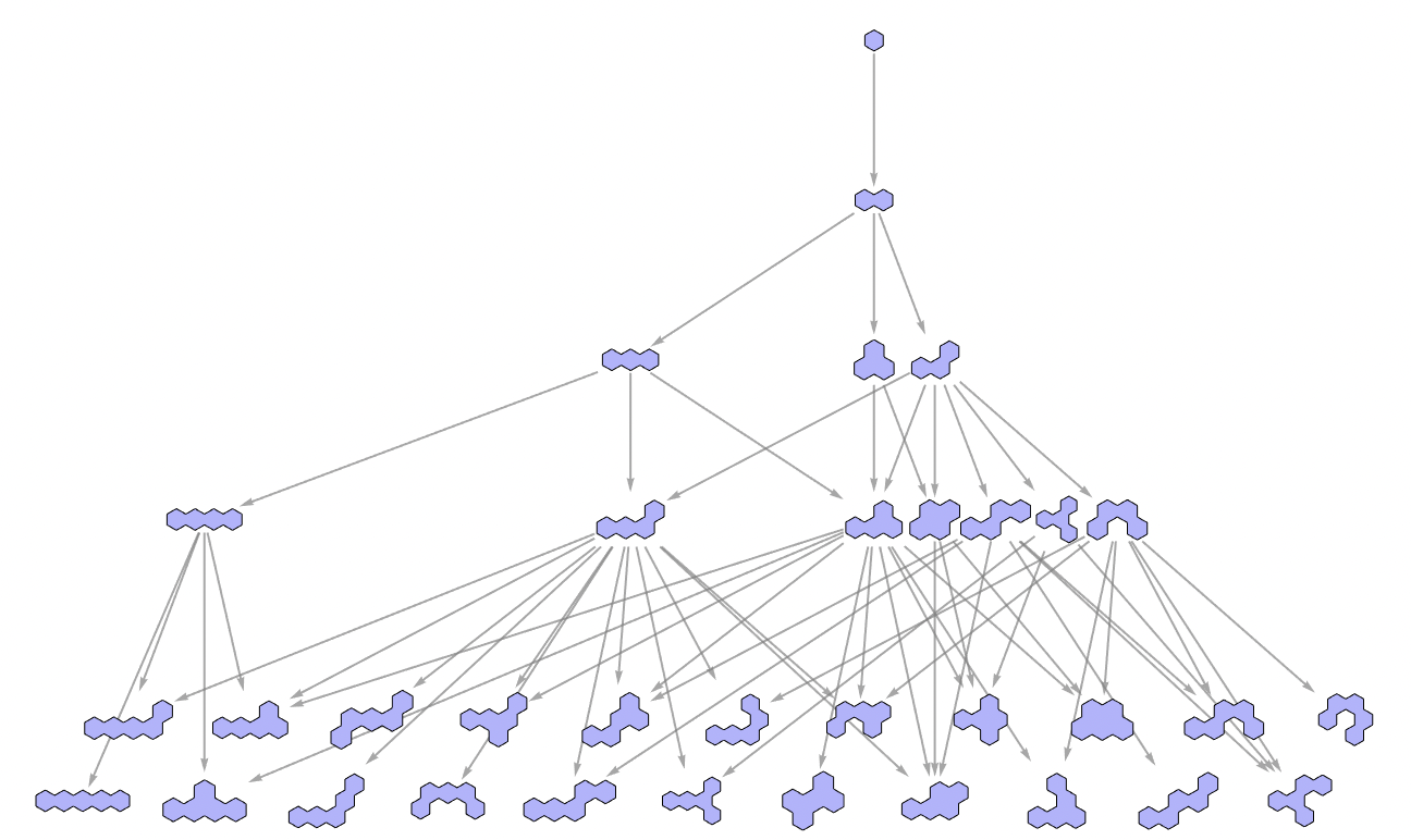
The pentahexes are found here on the fifth level (the two bottom-most rows in the image above). They are the set of 22 possible shapes (up to rotations and reflections) obtained by joining exactly five hexagons edge-to-edge. The reason we might care about pentahexes in particular is that 5 * 12 * 22 =1320 is quite close to 5 * 12 * 21 =1260, one less than the number of hexagons in the large substitution pattern:
(Length@ Nest[Union[Flatten[# /. InflateRep]] &, T[{0, 0, 0}, 1], 3] - 1)
Out[9]= 1260
We can guess that it's possible to cover a 1/12th slice of the 1260 hexagons by all 22 pentahexes because along lines of symmetry pentahexes do not generally contribute all of their hexagonal units to the total count. The details are not guaranteed to work out nicely, but as we shall see shortly they do anyways. Prepare to be amazed by fortunate numerical coincidences!
To clarify what's meant by "1/12 slice", we can actually make an AdjacencyGraph object depicting the structure of the hexagonal tiling, and then divide it up along its axes of symmetry:
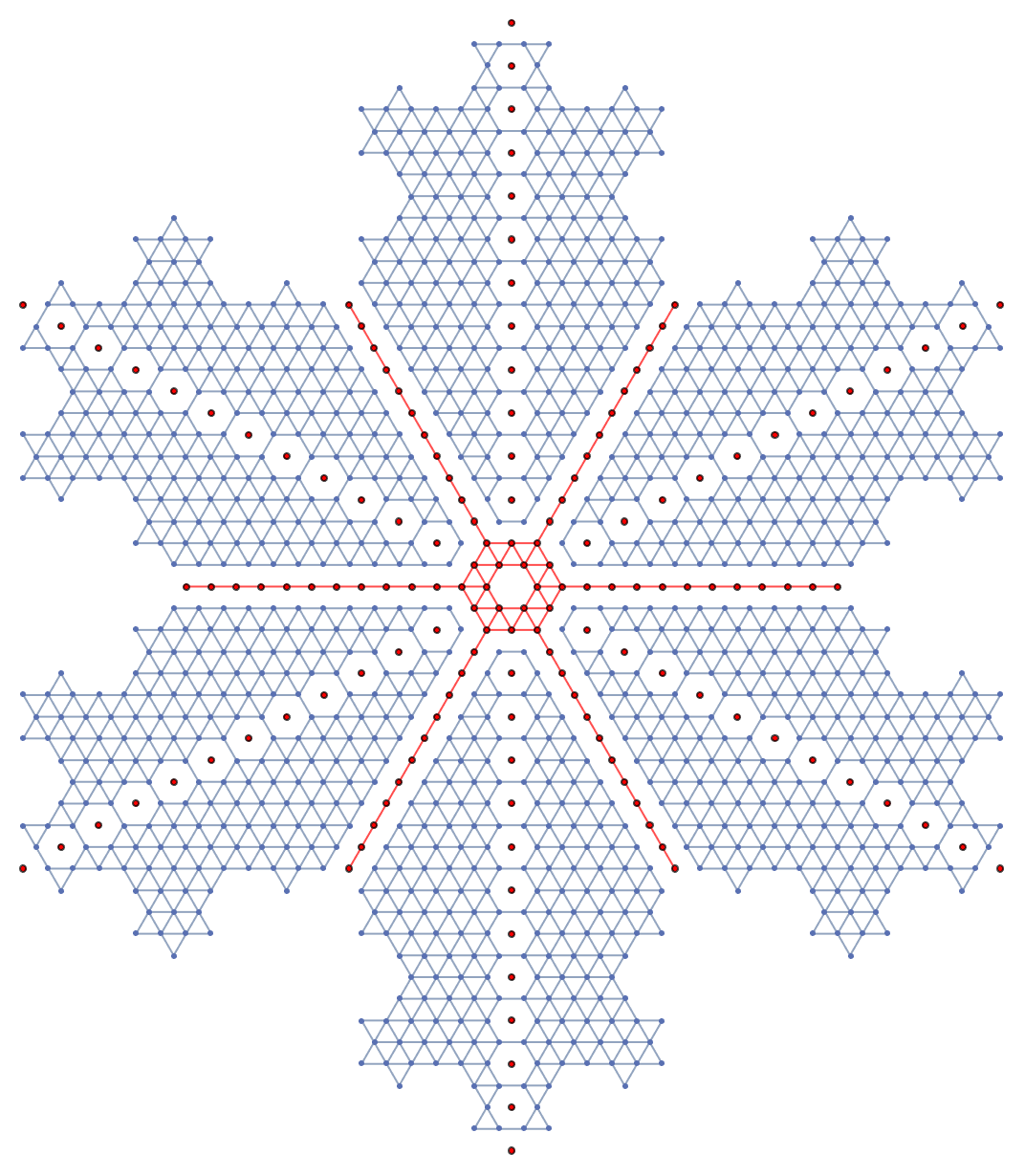
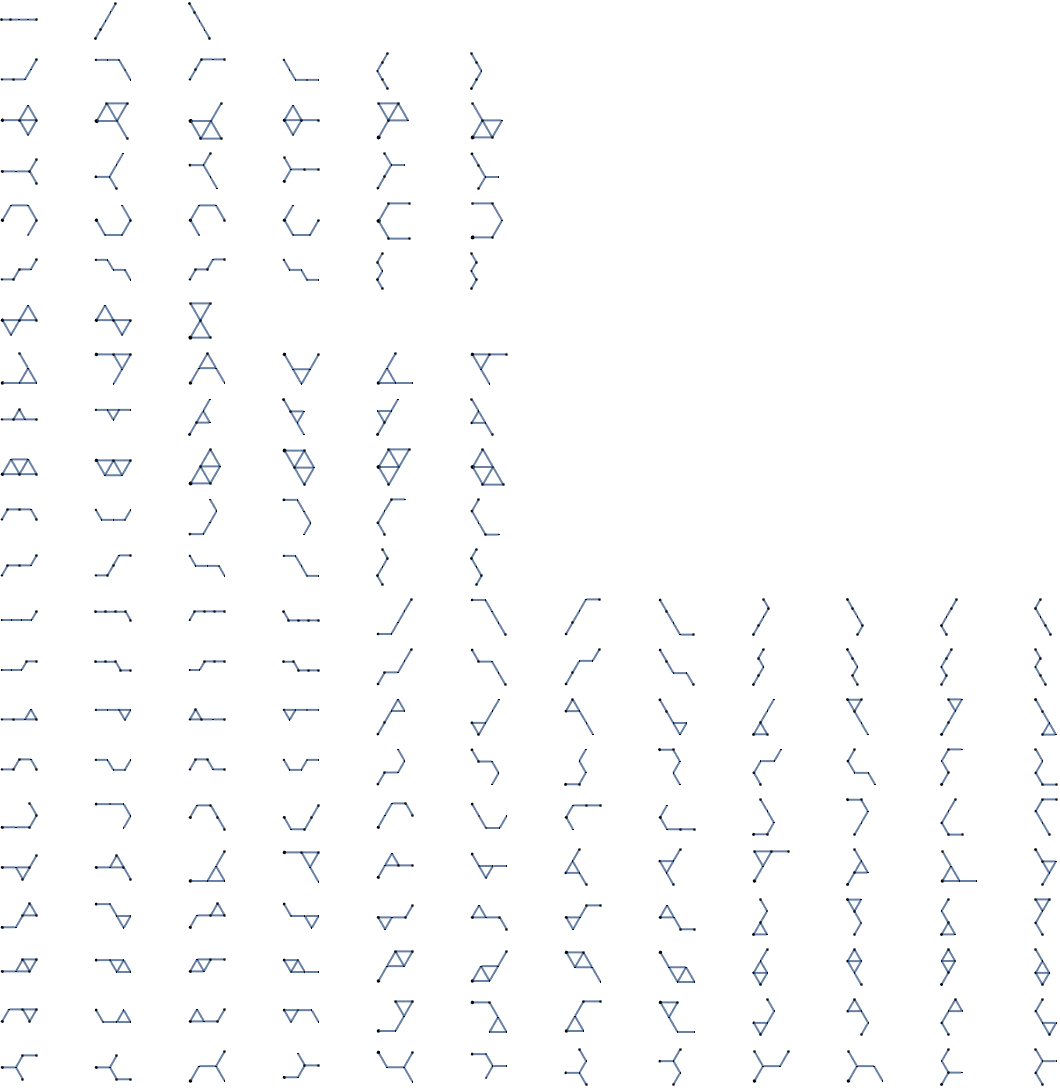
When covering the hexagonal tiling with pentahexes, we will want to keep all twelve symmetries. This means that pieces falling on a red vertex must have a reflection symmetry, and the local/global reflection axes must align. Of the 22 pentahexes, six have a plane of reflection symmetry passing through two hexagonal edges:
eSymPolyhexes = {
   {{0, 0, 0}, {0, 0, -1}, {0, 0, -2}, {0, 0, -3}, {0, 0, -4}},
   {{0, 2, 0}, {0, 1, 0}, {0, 0, 0}, {2, 0, 0}, {1, 0, 0}},
   {{0, -2, 0}, {0, -1, 0}, {0, 0, 0}, {-2, 0, 0}, {-1, 0, 0}},
   {{0, 0, 0}, {0, 0, -1}, {0, 0, -2}, {0, -1, -2}, {-1, 0, -2}},
   {{0, 0, 0}, {0, 0, -1}, {0, 0, -2}, {0, 1, 0}, {1, 0, 0}},
   {{0, 0, 0}, {0, 0, -1}, {0, 0, -2}, {0, -1, 0}, {-1, 0, 0}},
   {{0, 0, 0}, {0, 0, -1}, {0, 0, -2}, {0, 1, -2}, {1, 0, -2}},
   {{-1, 0, 1}, {-1, 0, 0}, {0, 0, 0}, {0, -1, 0}, {0, -1, 1}},
   {{1, 0, -1}, {1, 0, 0}, {0, 0, 0}, {0, 1, 0}, {0, 1, -1}},
   {{1, -1, 0}, {1, 0, 0}, {0, 0, 0}, {0, 1, 0}, {-1, 1, 0}},
   {{-1, 1, 0}, {-1, 0, 0}, {0, 0, 0}, {0, -1, 0}, {1, -1, 0}}
   };

Row[Map[Graphics[{Line[{{-5 symStar[[3]], 5 symStar[[3]]}}],
     EdgeForm[Thin], Lighter[Blue, .6],
     PolyhexPrimitive[# . symStar & /@ #]}, ImageSize -> 75] &,
  eSymPolyhexes, {1}],
 Spacer[3]]
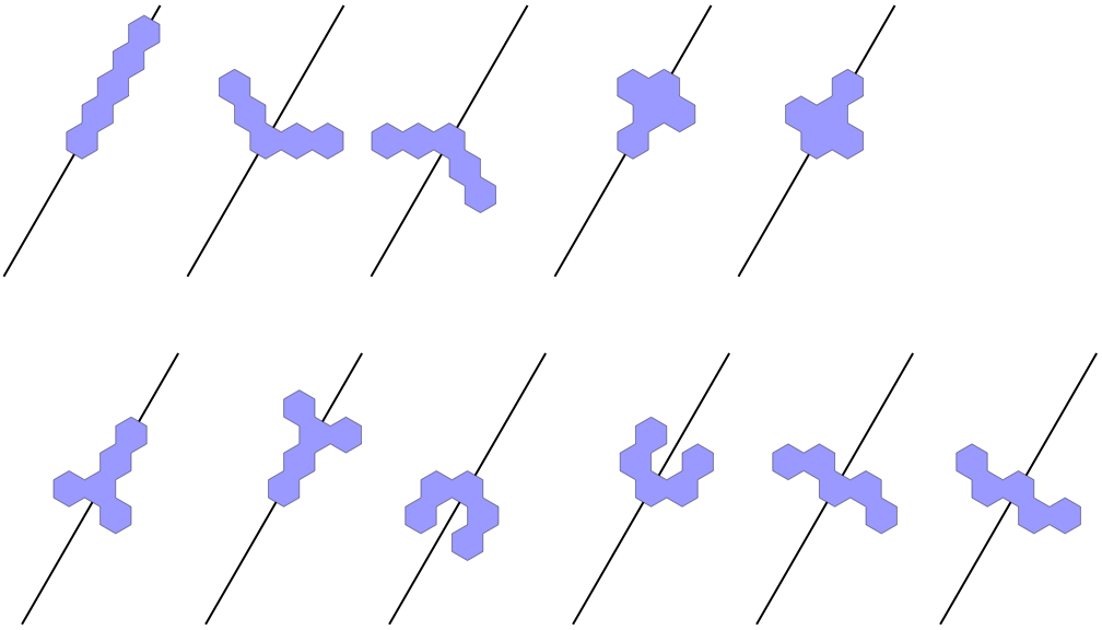
And five have a plane of reflection symmetry passing through two hexagonal vertices:
vSymPolyhexes = {
   {{0, 0, 1}, {0, 0, -1}, {0, 0, 0}, {0, 1, 0}, {0, -1, 0}},
   {{0, 0, -2}, {0, 0, -1}, {0, 0, 0}, {0, 1, 0}, {0, 2, 0}},
   {{0, 0, 2}, {0, 0, 1}, {0, 0, 0}, {0, -1, 0}, {0, -2, 0}},
   {{1, 0, -1}, {0, 0, -1}, {0, 0, 0}, {0, 1, 0}, {-1, 1, 0}},
   {{-1, 0, 1}, {0, 0, 1}, {0, 0, 0}, {0, -1, 0}, {1, -1, 0}},
   {{0, -1, -1}, {0, 0, -1}, {0, 0, 0}, {0, 1, 0}, {0, 1, 1}},
   {{0, 1, 1}, {0, 0, 1}, {0, 0, 0}, {0, -1, 0}, {0, -1, -1}},
   {{-1, 1, 0}, {-1, 0, 0}, {0, 0, 0}, {1, 0, 0}, {1, 0, -1}},
   {{1, -1, 0}, {1, 0, 0}, {0, 0, 0}, {-1, 0, 0}, {-1, 0, 1}}
   };


Row[Map[Graphics[{Line[{{{0, -3}, {0, 3}}}],
     EdgeForm[Thin], Lighter[Blue, .6],
     PolyhexPrimitive[# . symStar & /@ #]},
    PlotRange -> {{-2, 2}, {-3, 3}},
    ImageSize -> 75] &, vSymPolyhexes, {1}],
 Spacer[3]]
All symmetry axes have exactly 13 points along any direction from the centroid. In the first set of six pieces, we should be able to count uniquely up to thirteen by stacking along the axis because some of the pieces have numerous hexagons falling on axis. The same isn't true for the second set, in which every piece has exactly one hexagon on axis. This problem of not having enough pieces for the vertical is likely to be a deal-breaker for some connoisseurs of exact tiling problems, but if they stop reading now and miss out what's to follow, they only have their own self-doctrine clinging to thank!
We will accept a few repeats on the vertical diagonal. We can then see plainly that we will cover 13 * 2 slots on a 1/12 slice (including the boundary), and that the first two pieces near the origin are uniquely defined, a V followed by a weird T, as well as the outermost piece, an inverted weird T. This takes us from 105 slots to 79. The second count is a bit more difficult, but if we check integer partitions:
Select[IntegerPartitions[13], SameQ[Union[#], {1, 3, 5}] &]
Out[18]= {{5, 3, 3, 1, 1}, {5, 3, 1, 1, 1, 1, 1}}
We find a solution {5,3,3,1,1} which uses 5 out of 6 pieces and will occupy 19 slots. This reduces the count of open slots from 79 to 60. In this holiday Miracle, 5 divides 60 evenly into 12, the exact number of asymmetric pieces plus one more for whichever through-edge symmetric piece gets left out of the diagonal boundary.
What we have now is a well-formed exact cover problem that isn't too different from the original "Scott's pentomino" problem discussed in Knuth's arxiv article. The difference is that the previous problem about placing 12 pentominoes in a chess board essentially has one fixed boundary condition, but in this new problem about 12 polyhexes we will have a variable number of oddly-shaped boundary conditions. But If we can get even one solution with all 22 pentahexes in a 1/12 slice, we know that roto-reflecting through the hexagonal template will also get us all orientations of all pieces.
The diagonal is easier to work with and less ambiguous how to filter. The first piece near the origin must be a straight line, and the last piece can not be a C with its end-points pointing out. Between these two pieces we must choose a few more consistently (meaning they can't overlap or leave impossible boundaries). The who-follows-who rules can be written in an Association:
eSymLens = {5, 1, 1, 3, 3, 3, 3, 1, 1, 1, 1};

eSymSeqRules = Association[MapIndexed[#2[[1]] -> #1 &,
    Outer[Function[{ind1, ind2},
      Function[{vertices1, vertices2},
        If[And[! SameQ[ind1, ind2], SameQ[
           Intersection[vertices1, vertices2], {}]],
         ind2, Nothing]][
       # . symStar & /@ eSymPolyhexes[[ind1]],
       Dot[# + {0, 0, -eSymLens[[ind1]]},
          symStar] & /@ eSymPolyhexes[[ind2]],
       ind2]], Range[11], Range[11], 1]]];
(* minor fix needed *)
eSymSeqRules[11] = eSymSeqRules[11][[1 ;; 7]];

eSymSeqRules

Out[22]= <|1 -> {2, 3, 4, 5, 6, 7, 8, 9, 10, 11},
 2 -> {1, 4, 5, 7, 9}, 3 -> {1, 2, 4, 5, 6, 7, 9, 10, 11},
 4 -> {1, 2, 3, 5, 6, 7, 9, 10, 11},
 5 -> {1, 2, 3, 4, 6, 7, 8, 9, 10, 11},
 6 -> {1, 2, 3, 4, 5, 7, 8, 9, 10, 11}, 7 -> {1, 2, 4, 5, 9, 10},
 8 -> {1, 2, 3, 4, 5, 6, 7, 9, 10, 11}, 9 -> {1, 4, 7},
 10 -> {1, 2, 4, 5, 7, 9}, 11 -> {1, 2, 4, 5, 6, 7, 9}|>
This data then gets sent to an iterator, and we can even track topology of results finding process by plotting the breadth-first search tree:
IterateSymEdge[rules_, lens_][path_] := Select[Map[
   Append[path, #] &,
   Complement[rules[Last[path]
     ], path]], Total[lens[[#]]] <= 13 &]

geSym = ResourceFunction["NestWhileGraph"][
  IterateSymEdge[eSymSeqRules, eSymLens],
  {{1}}, UnsameQ @@ # &, 2]
The results we care about can be filtered out as follows:
With[{eSymSeqs = DeleteCases[Select[VertexList[geSym],
      Total[eSymLens[[#]]] == 13 &], {__, 9}]},
  ueSymSeqs = eSymSeqs[[Flatten[
      Position[Apply[Or, #] & /@ Outer[SubsetQ[#1, #2] &, eSymSeqs,
         {{2, 3}, {4, 5}, {6, 7}, {8, 9}, {10, 11}}, 1], False]
      ]]]];
 Length[ueSymSeqs]

Out[26]= 440
And we find only 440 valid boundaries. This is great because 500^2 = 250K is a totally reasonable number for a super-fast algorithm that gets results in seconds (and still an approachable number even if timings leave something to desire--more on that later).
Now we just need to do something similar with the second set of symmetric polyhexes, but in this case what to accept is not as clear, and somewhat subject to taste. The leader-follower rules are:
vSymSeqRules = Association[MapIndexed[#2[[1]] -> #1 &,
   Outer[Function[{ind1, ind2},
     Function[{vertices1, vertices2},
       If[And[! SameQ[ind1, ind2],
         SubsetQ[Union[vertices1, vertices2],
          # . symStar & /@ {{0, 1, 0}, {0, 0, -1}} ],
         SameQ[
          Intersection[vertices1, vertices2], {}]],
        ind2, Nothing]][
      # . symStar & /@ vSymPolyhexes[[ind1]],
      Dot[# + {0, 1, -1},
         symStar] & /@ vSymPolyhexes[[ind2]],
      ind2]], Range[9], Range[9], 1]]]

Out[27]= <|1 -> {2, 4, 6, 8, 9}, 2 -> {4}, 3 -> {1, 5, 7},
 4 -> {2, 6, 8}, 5 -> {1, 3, 7}, 6 -> {2, 4, 8, 9}, 7 -> {1, 5},
 8 -> {1, 7}, 9 -> {1, 5, 7}|>
Again these such rules go through an iterator to create a graph (which this time is just too large to depict).
IterateSymEdge[rules_][path_] := Select[Map[
   Append[path, #] &, rules[Last[path]]],
  Max[Tally[#][[All, -1]]] < 3 &
  ]

vSymSeqs =   Select[VertexList@NestGraph[IterateSymEdge[vSymSeqRules], {{2}}, 12],
   And[Length[#] == 13, Last[#] == 5,
     Length@Union[Floor[(# + 1)/2]] == 5] &];

Length[vSymSeqs]

Out[30]= 1495
A total of 1495 isn't too high, but we can cut again by counting rotations as unique, then we get only 391 boundary conditions to search through:
vSymSeqsMax = Select[vSymSeqs, Length[Union[#]] == 9 &];
Length[vSymSeqsMax]
Out[32]= 391
The next question regards how many of the 440*391 paired boundary conditions are mutually consistent. Before diving into that, let's make some more utilities to plot and see what we already have as well as what may be problematic. For example, here's one pair that will not work:
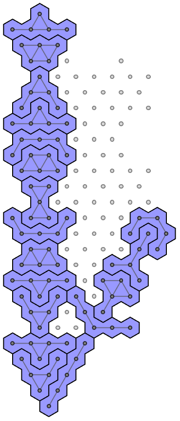
We need a test that detects overlaps while filtering out candidates that divide interior space into parts which can't be tiled by pentahexes (as above). Here it is, but it may take more than a half hour to generate the data:
CheckComponents[ind1_, ind2_, tf_ : True] := Module[{
   g0 = BoundariesGraph[ind1, ind2], gs},
  If[VertexCount[g0] == 90,
   gs = WeaklyConnectedGraphComponents[
     VertexDelete[gOneSlice,
      Alternatives @@ (VertexList@g0)]];
   If[AllTrue[gs, Mod[VertexCount[#], 5] == 0 &],
    If[tf,
     {ind1, ind2} -> GraphUnion @@ gs,
     {ind1, ind2}],
    Failure["Disconnect",  <||>]],
   Failure["Overlap",  <||>]]
  ]

(*AbsoluteTiming[bcRes=Outer[CheckComponents[#1,#2,False]&,
Range[440],Range[391],1];]*)

(*Iconize[Select[Catenate[bcRes],!FailureQ[#]&]]*)
viable = Icon
 Length@viable

Out[42]= 61772
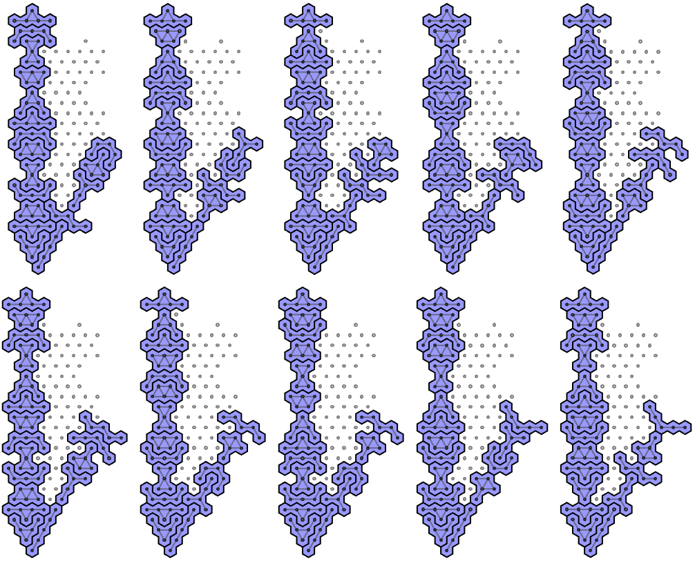
It turns out there are 61,772 viable boundary conditions. Here is a short random sample showing some of the different possibilities:
Grid[Partition[With[{bg1 = BoundariesGraph @@ #},
     Show[Graphics[{Lighter[Blue, .6], EdgeForm[Black],
        PolyhexPrimitive /@ WeaklyConnectedComponents[bg1],
        LightGray, EdgeForm[Gray],
        Disk[#, 1/10] & /@
         Complement[VertexList[gOneSlice], VertexList[bg1]]}],
      Graph[bg1, EdgeStyle -> Darker@Gray, VertexStyle -> Gray],
      ImageSize -> {Automatic, 200}]] & /@
   With[{rand = SeedRandom[134134]}, RandomChoice[viable, 10]], 5]]
There is also a small minority of disconnected cases, only 1326, some of which are depicted here:
 (* this is also kinda slow *)
disconnected = Select[viable,
   Length[WeaklyConnectedComponents[VertexDelete[gOneSlice,
        Alternatives @@ VertexList[BoundariesGraph @@ #]]]] > 1 &];

Grid[Partition[With[{bg1 = BoundariesGraph @@ #},
     Show[Graphics[{Lighter[Blue, .6], EdgeForm[Black],
        PolyhexPrimitive /@ WeaklyConnectedComponents[bg1],
        LightGray, EdgeForm[Gray],
        Disk[#, 1/10] & /@
         Complement[VertexList[gOneSlice], VertexList[bg1]]}],
      Graph[bg1, EdgeStyle -> Darker@Gray, VertexStyle -> Gray],
      ImageSize -> {Automatic, 200}]] & /@
   With[{rand = SeedRandom[982374]}, RandomChoice[disconnected, 10]],
  5]]
Most of them can be discarded on inspection just by noticing where they would require a duplicate symmetric piece interior (against rules spelled out above). But some of these might be good examples to explore, especially because they seem to close off a second hexagonal form around the interior:
To make the exact cover matrix, we have to be somewhat careful about which extra symmetric piece gets included with the set of 11 asymmetric pieces. When were done worrying about indices, the sorted pentahex data looks as follows:
When constructing the cover matrices, we will always choose one row out of the first six to combine with the last 11 rows, while ignoring the middle five rows. This is done by a single function, and we then send the reduced data to another function that constructs the exact cover matrix. Those functions are:
PentahexHand[viableInds_] := Part[sortedPentahexData,
  Join[Range[12, 22], Complement[Range[6],
    Ceiling[(ueSymSeqs[[#1]] + 1)/2
       ] & @@ viableInds]]
  ]

PentahexExactCoverMatrix[viable_] :=
 Module[{hand = PentahexHand[viable],
   domainVertices = VertexList[Last[CheckComponents @@ viable]]},
  Catenate[MapThread[Function[{piece, offsets},
     Join[piece, #] & /@ offsets],
    {IdentityMatrix[12],
     Catenate[If[SubsetQ[domainVertices, #],
             Normal@SparseArray[Map[Rule[#, 1] &,
                Flatten[Position[domainVertices, #] & /@ #]], {60}]
             , Nothing] & /@ Outer[Plus, domainVertices, #, 1] & /@ #
        ] & /@ hand}]]
  ]
Once cover matrices can be made programmatically, the real fun begins discovering which matrices have good solutions and if so how many. For example, here's one:
AbsoluteTiming[res = ResourceFunction["FindExactCover"][
PentahexExactCoverMatrix[{119, 1} ], 1];]
Out[63]= {64.2982, Null}
SymmetrizeGraphs[g1_, g2_] := GraphUnion[
RotoReflect[{1, 1}][g1],
RotoReflect[{1, 1}][g2],
RotoReflect[{1, -1}][g2]
]
weights = Association[Flatten[
Nest[# /. InflateRep &, T[{0, 0, 0}, 1], 3]
] /. T[x_, c_] :> Rule[x . symStar, c]];
DepictExactCover[inds_, res_] := Module[
{g1, g2, vertices, components, colors, colorfun},
g1 = BoundariesGraph @@ inds;
vertices = VertexList[Last[CheckComponents @@ inds]];
g2 = Graph[Catenate[EdgeList[
NearestNeighborGraph[vertices[[# - 12 & /@ Flatten[
Rest@Position[#, 1]]]]]] & /@ res]];
colorfun = Function[{Lighter[Lighter@Blue,
(4 - Min[Max[Last /@ Tally[Lookup[weights, #]]], 3])/4
], EdgeForm[Thin]}];
components = WeaklyConnectedComponents[SymmetrizeGraphs[g1, g2]];
Graphics[Append[MapThread[Append[#1, #2] &, {
Map[colorfun, components],
Map[PolyhexPrimitive[#] &, components]}],
{Lighter[Blue, 3/4], EdgeForm[Thin],
Polygon[CirclePoints[{0, 0}, {1/Sqrt[3], Pi/6}, 6]]}],
ImageSize -> 600]
]
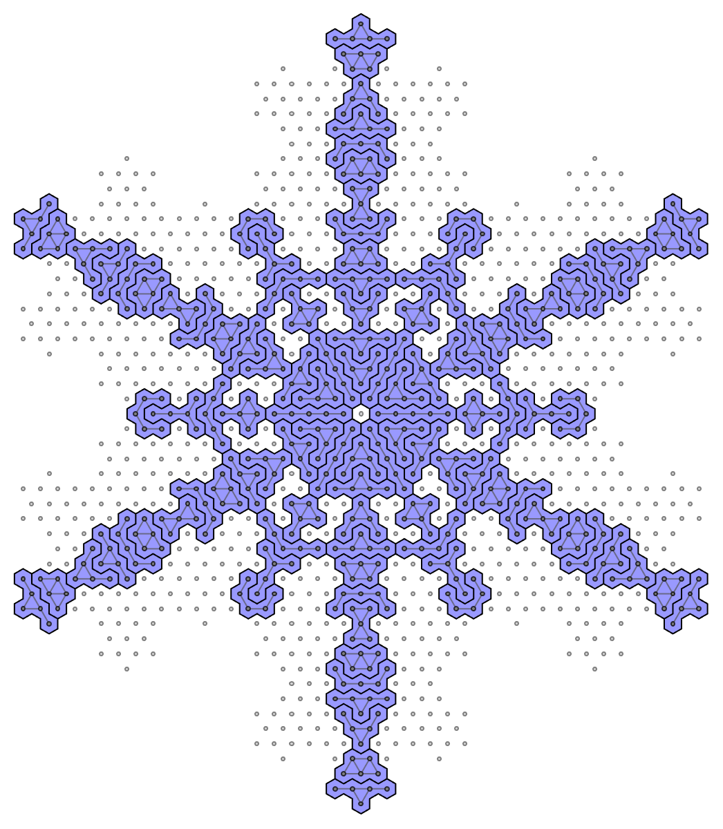
DepictExactCover[{119, 1}, res]
Wow looks pretty good already, if I may say so myself! Even though we are interested in just one particular solution, were are also interested in all possible solutions, and the statistics that describe them.
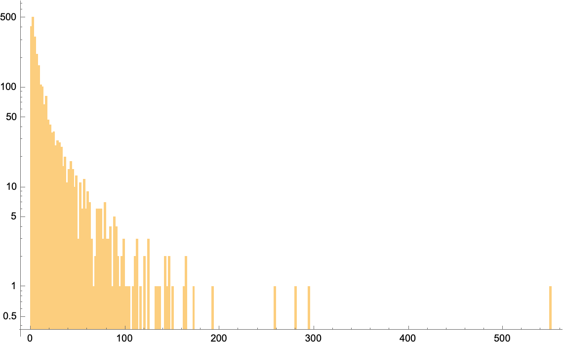
The code is omitted here, but we're currently running an extensive search that' already turned up 10's of thousands of unique and special results. I just checked the exact number so far is 35,221 and still ticking. Here's a log plot of the histogram for number of results per cover matrix:
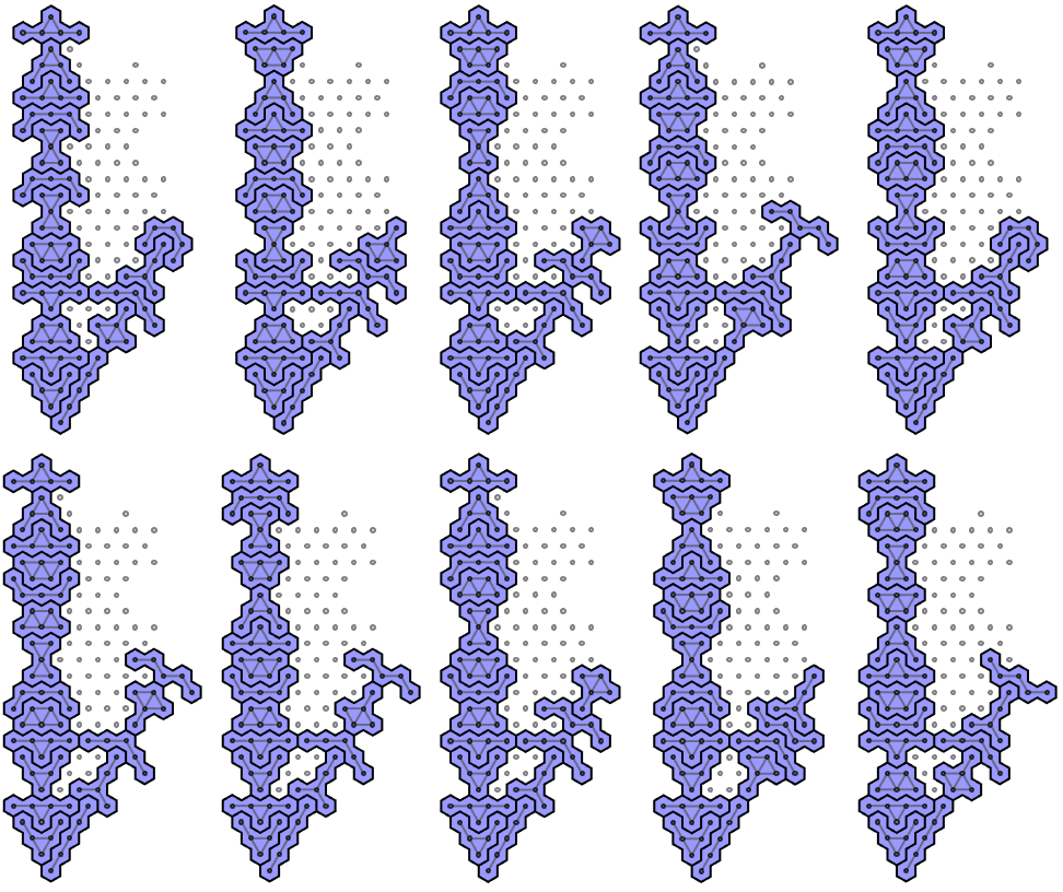
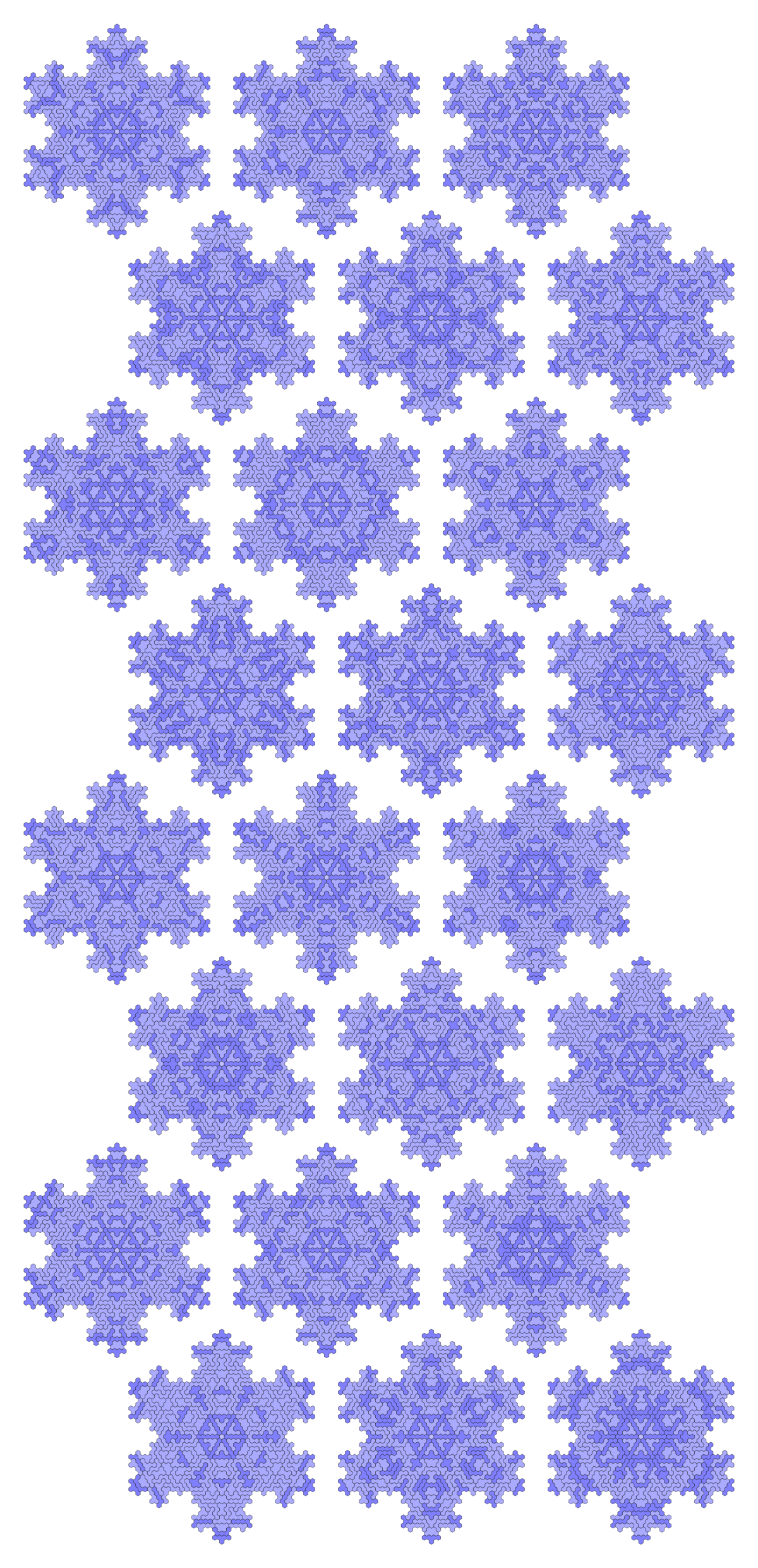
This data suggests we might ultimately find up to 1 million results, but I think the final count will fall short of that. While we are waiting (maybe a few more months, or until code is better optimized), here is a random sampling of all results:
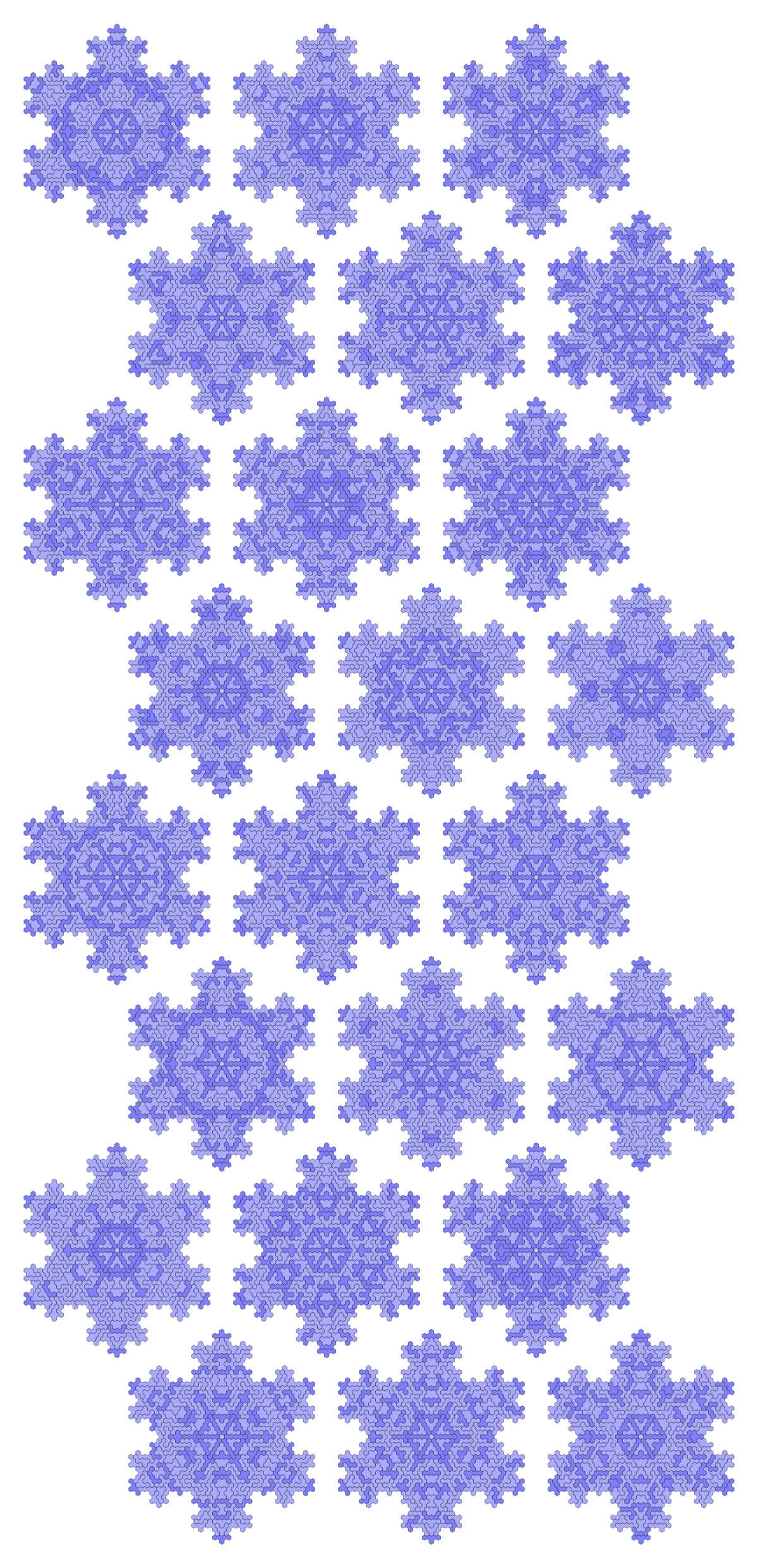
Why not? Here's another Random sampling of all results:
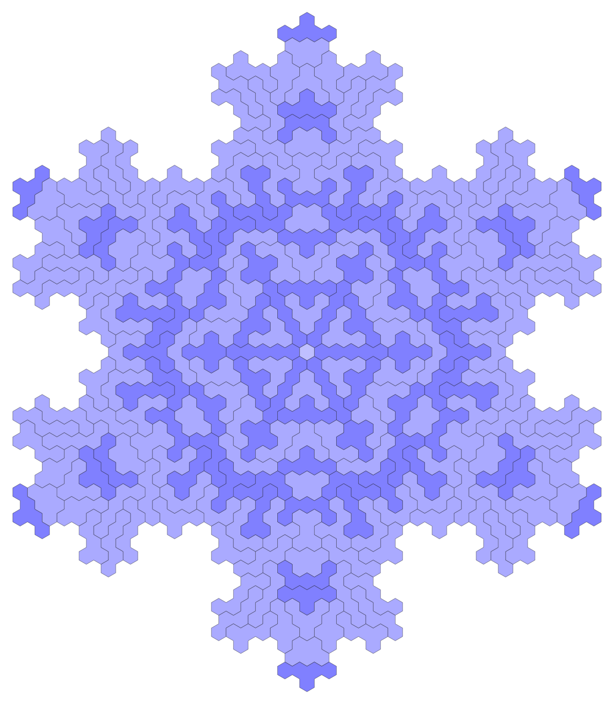
We could go on to make thousands of similar plots without repeating ourselves, but here will save space from doing so. Instead, we just make an extra height map that could be the setting for a game of hexagonal checkers in 2.5 dimensions:
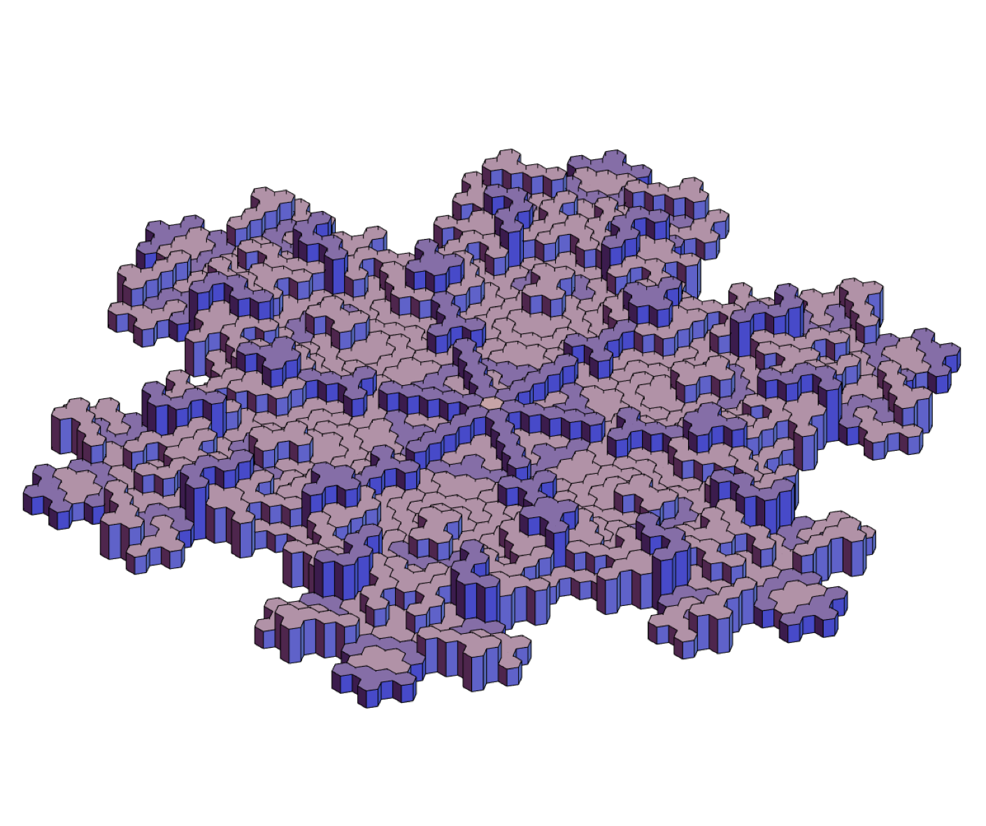
Just imagine hopping some marbles around that landscape!
In summary, we have more than enough results to start making holiday cards, but we need to do a bit more work before we can answer the "how many exist?" number theory question (most practical people don't care anyways). In subsequent posts we may explain just why this example is so well tuned to Dancing Links, but for now we leave it up to the audience to verify that other methods are much slower.


