• Introduction

Linear algebra is a branch of mathematics that studies vectors, vector spaces, linear representations, and systems of linear equations. Analytic geometry is its expression and is itself a central connective tissue of modern mathematics, particularly through the abstract concept of vector space that can model many different problems encountered in practice.

It is common practice to approximate non-linear phenomena with linear models (linearisation) in order to enable the application of linear algebra methodologies. This 'linearity' refers to the fact that these methodologies are applied to sets of functions which in their formula contain only polynomials of degree one or zero and describe relations between n-dimensional vectors. These functions are also called linear functions because they are visually represented by straight lines in analytical geometry.

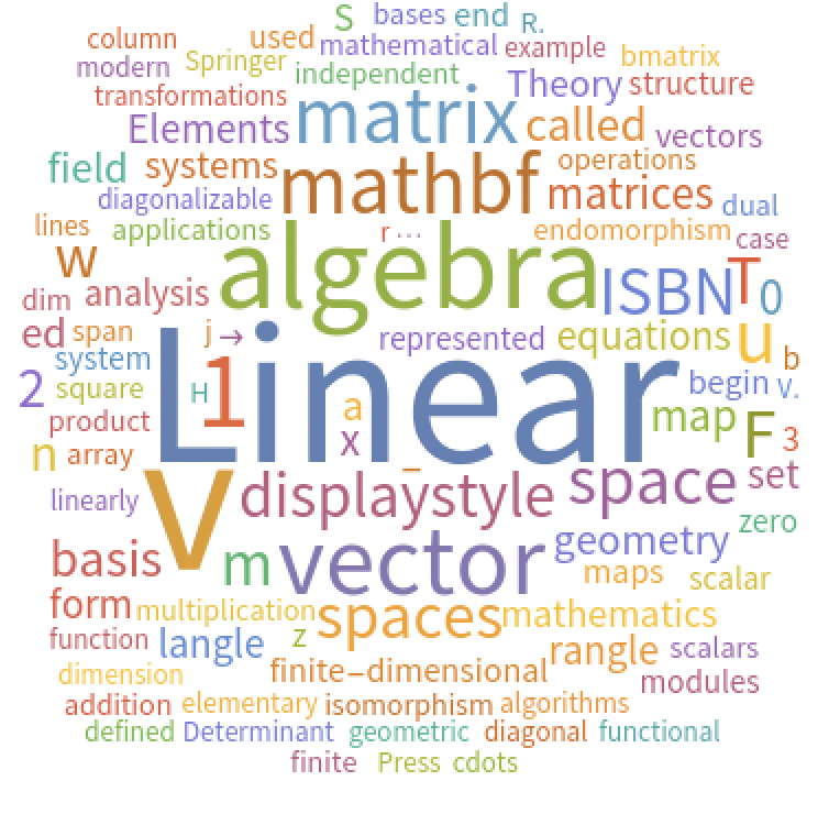
WordCloud[WikipediaData["Linear Algebra"]]

• Linear systems

In mathematics, the theory of linear systems is the basis and a fundamental part of linear algebra, a subject used in most parts of modern mathematics. Computational algorithms for finding solutions are an important part of numerical linear algebra and play a prominent role in engineering, physics, chemistry, computer science, and economics. A system of nonlinear equations can often be approximated by a linear system (see linearization), a useful technique when constructing a mathematical model or computer simulation of a relatively complex system.

Very often, the coefficients of the equations are real or complex numbers and solutions are sought in the same set of numbers, but the theory and algorithms apply to coefficients and solutions in any domain. For solutions in an integral domain, such as the ring of integers, or in other algebraic structures, other theories have been developed, see Linear equation over a ring. Integer linear programming is a collection of methods for finding the "best" integer solution (when there are many). Gröbner basis theory provides algorithms when the coefficients and unknowns are polynomials. Also, tropical geometry is an example of linear algebra in a more exotic structure. ***

• Solving a linear system with the Solve command

- Problem 1 One hundred and thirty-six tourists were transported in 10 buses of 12 and 16 seats. How many buses were there of each type?

Solution

We denote $x,y$ and construct the equations of the system.

Let $x$ be the number of buses with 12 seats and $y$ of 16 seats.

We have the following system: $$x + y = 10\\ 12 x +16 y =136 $$

ssys={x+y==10,12x+16y==136};
sol=Solve[sys,{x,y}]

The solution will be $x=6$ and $y=4$.

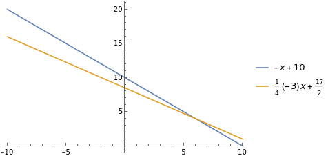
To solve the system graphically we plot the lines $(\varepsilon_1)$ and $(\varepsilon_2)$, represented by the two equations, on a common axis system and consider the coordinates of their common points as the solution of the system.

In particular, we have the following cases:

1. When the lines $(\varepsilon_1)$ and $(\varepsilon_2)$ intersect, then the system has a unique solution. This solution is the coordinates of their intersection point M(x0,y0)
2. When the lines $(\varepsilon_1)$ and $(\varepsilon_2)$ are parallel, so the system has no solution.
3. When the lines $(\varepsilon_1)$ and $(\varepsilon_2)$ are identical, then they have infinite common points, namely all points of the common line, i.e. the system has infinite solutions. We then say that the system is indefinite.

So, we can solve the system graphically with the following command:

Plot[{-x+10,-(3/4)x+17/2},{x,-10,10},PlotLegends->"Expressions"]

***

• Solving a linear system with the $LinearSolve$ command

- Problem 2 Find the ages of the mother and daughter if today they differ by 35 years and after 5 years the mother's age will be twice the age of her daughter.

Solution Let $x$ be the mother's age and $y$ be the daughter's age. After 5 years, the mother's age will be $x +5$ and the daughter's age will be $y +5$. So we get a system of the form:

$$ x-y = 35\\ x-2y = 5$$

First, we write the coefficient table: $A= \begin{pmatrix} 1 & -1 \\ 1 & -2 \end{pmatrix}$. Then, we write the constants on the right-hand side as a matrix: $b= \begin{pmatrix} 35 \\ 5 \end{pmatrix}$. Finally, we solve the system using the command $Linear Solve$. In the code of Mathematica, the above system will be written using the \en LinearSolve\gr command as follows:

A={{1,-1},{1,-2}};
MatrixForm[A]
b={35,5};
MatrixForm[b]
LinearSolve[A,b] 

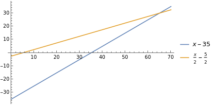
Solve the system graphically with the following command:

Plot[{x-35,(1/2)x-(5/2)},{x,0,70},PlotLegends->"Expressions"]

• Solving a linear system with the $RowReduce$ command

In linear algebra, Gaussian elimination or Gauss elimination is an algorithm for solving systems of linear equations. It is usually understood as a sequence of operations performed on the rows of the coefficient matrix. The algorithm essentially converts the augmented matrix of the system into a scalar matrix, which is also used to find the order of the matrix, calculate the horizon of a matrix, and calculate the inverse square matrix (when available). The method was named after Carl Friedrich Gauss (1777-1855), although it was already known by Chinese mathematicians as early as 179 BC).

The basic idea of the algorithm is that the rows of the matrix can be modified using some elementary transformations, but without changing the space of its columns and therefore the solutions of the system. The algorithm modifies the matrix up to its lower left corner by filling it with as many zeros as possible. There are three types of allowed elementary actions:

1. Opposition of two lines,
2. Multiplying a line by a non-zero number.
3. Adding a multiple of a line to another line

Using these actions, each table can be converted to an upper triangular table in scalar form (or even in scalar reduced form). This final table form is unique, in other words, it is independent of the sequence of actions used. The above processes in Mathematica are done with the $RowReduce$ command. Let's look at a simple implementation of it.

- Problem 3 Solve the following system: $$x - 2y = 6 \\ 3x + 4y = 8$$

Solution First, we write the augmented table: $B= \begin{pmatrix} 1 & -2 & 6 \\3 & 4 & 8 \end{pmatrix}$ Then we adapt the Gaussian elimination with the $RowReduce$ command and we end up with the matrix $B= \begin{pmatrix} 1 & 0 & 4 \\ 0 & 1 & -1 \end{pmatrix}$.

The last column represents the solution of the system.

The above system will be written with the command $Rowreduce$ as follows:

B={{1,-2,6},{3,4,8}};
MatrixForm[B]
RowReduce[B]
MatrixForm[%]

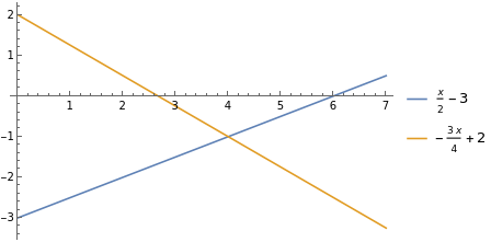
Solve the system graphically with the following command:

Plot[{(1/2)x-3,(-3/4)x+2},{x,0,7},PlotLegends->"Expressions"