Recently we were looking back on a nice talk that was given here by Richard Gass, and also observing that we now have more options how to write the code for analysis of video data. The new function VideoMapList is a really nice way to transform video data into numeric form. Potentially it is more transparent and less prone to unexpected failures than ImageFeatureTrack. The purpose of this memo is to get into the details how to use VideoMapList. It does take a bit of thought and well-prepared data.

Here's a data set, which was collected with the function Binarize in mind. It can be ripped off youtube fairly easily with a service such as this, then imported to a Mathematica session as:

vidData = Video["~/. . . /Physics/Data/pendulum.mp4"]; 

For each frame, we can Binarize to isolate the white spot, and prune any noise using NearestNeighborGraph + WeaklyConnectedComponents. The functional form is:

ExtractPosition[frame_, cut_ : 0.9
  ] := Reverse[Mean[First[ReverseSortBy[
     WeaklyConnectedComponents[
      NearestNeighborGraph[
       Position[ImageData[
         Binarize[frame, cut]], 1]]
      ], Length]]]]

Usage of Mean here is a bit expedient, but in this memo we're going for simplicity, not exactitude. The function ExtractPosition is then mapped as follows:

data = VideoMapList[ExtractPosition[#Image] &, vidData];

The output data should be a circular locus of Cartesian points. I don't know if FindFit can be adapted to extract the centroid and radius, so I just use Minimize instead:

FitCircle[data_, rot_ : 50] := Module[
  {diameters, diameter, fitFun},
  diameters = Apply[Subtract, -MinMax[Part[
         data . N[RotationMatrix[Pi/rot #]], All, 1]
        ]] & /@ Range[rot];
  diameter = Mean[diameters];
  fitFun = N[Total[Abs[EuclideanDistance[{x, y},
          #] - diameter/2] & /@ data]];
  {{StandardDeviation[diameters]/2, r -> diameter/2},
   Minimize[fitFun, {x, y}] }]

AbsoluteTiming[
 fitRes = FitCircle[data]
 ]

Out[]= {22.0165, {
{0.0714379,  r -> 103.092}, 
{3163.48, {x -> 264.781, y -> 146.438}}}}

We can then check the fit by inspection:

Show[
 ListPlot[Map[(# - {264.781, 146.438})/103.092 &, data]],
 Graphics[{Opacity[0], EdgeForm[Directive[Red]], Disk[{0, 0}, 1]}],
 PlotRange -> {{-1.1, 1.1}, {-1.1, 1.1}},
 AspectRatio -> 1
 ]

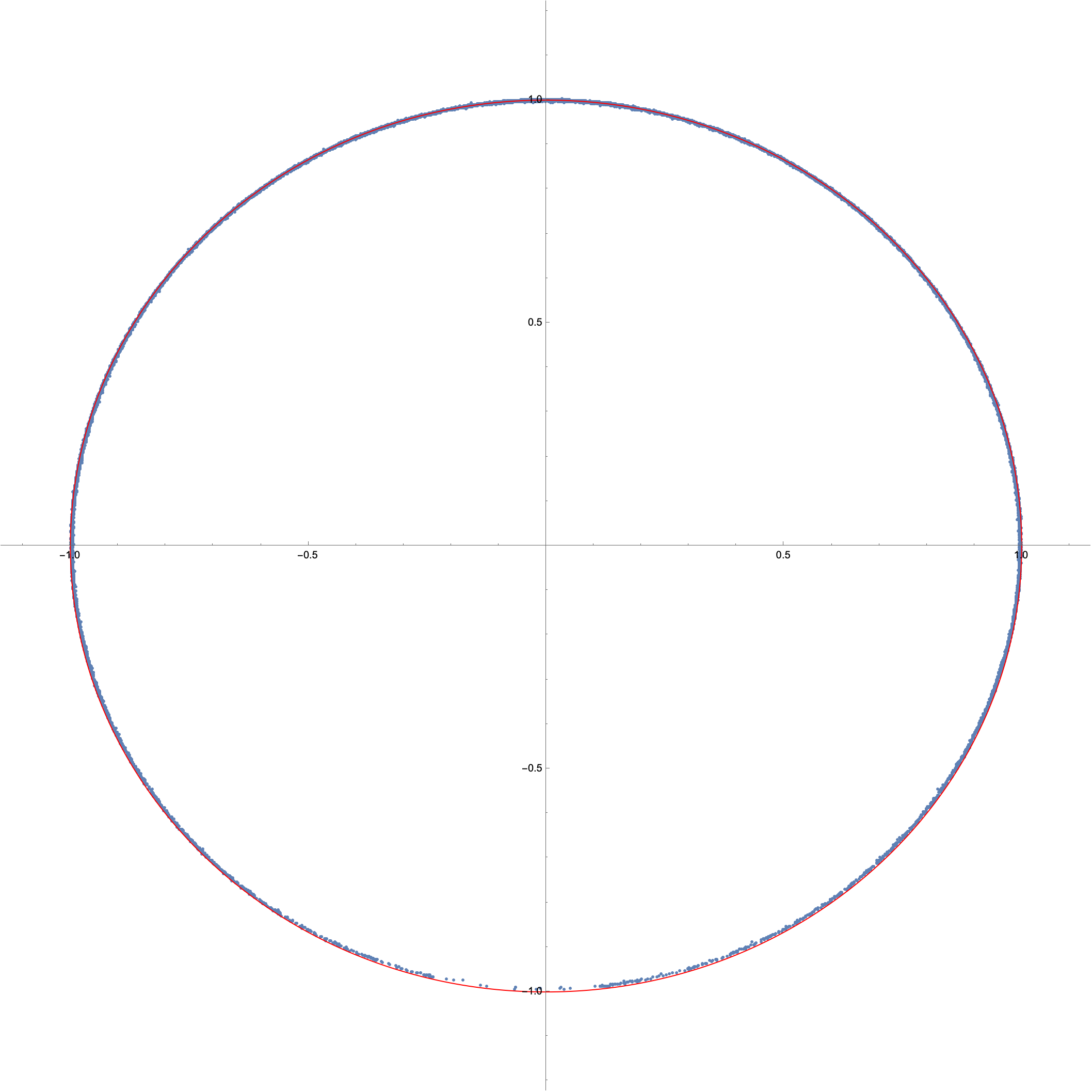
Looks pretty good, except possibly around the high end (bottom of plot, actually), where we may be seeing some wiggle room as the pendulum inverts. Nothing too substantial though. The remaining parameter, angular offset, needs to be found in order to tare the timeseries data:

TareData[data_, fitRes_,
  cut1_ : 200, cut2_ : -2000
  ] := Module[{cent, data2, tare},
  cent = {x, y} /. fitRes[[2, 2]];
  data2 = Apply[ArcTan[#2, #1] &,
      (# - cent)] & /@ data;
  tare = ReplaceAll[x, Minimize[Total[
       Abs[data2[[cut1 ;; cut2]] - x]], x][[2]]];
  data2 - tare
  ]

angleTimeseries = TareData[data, fitRes];

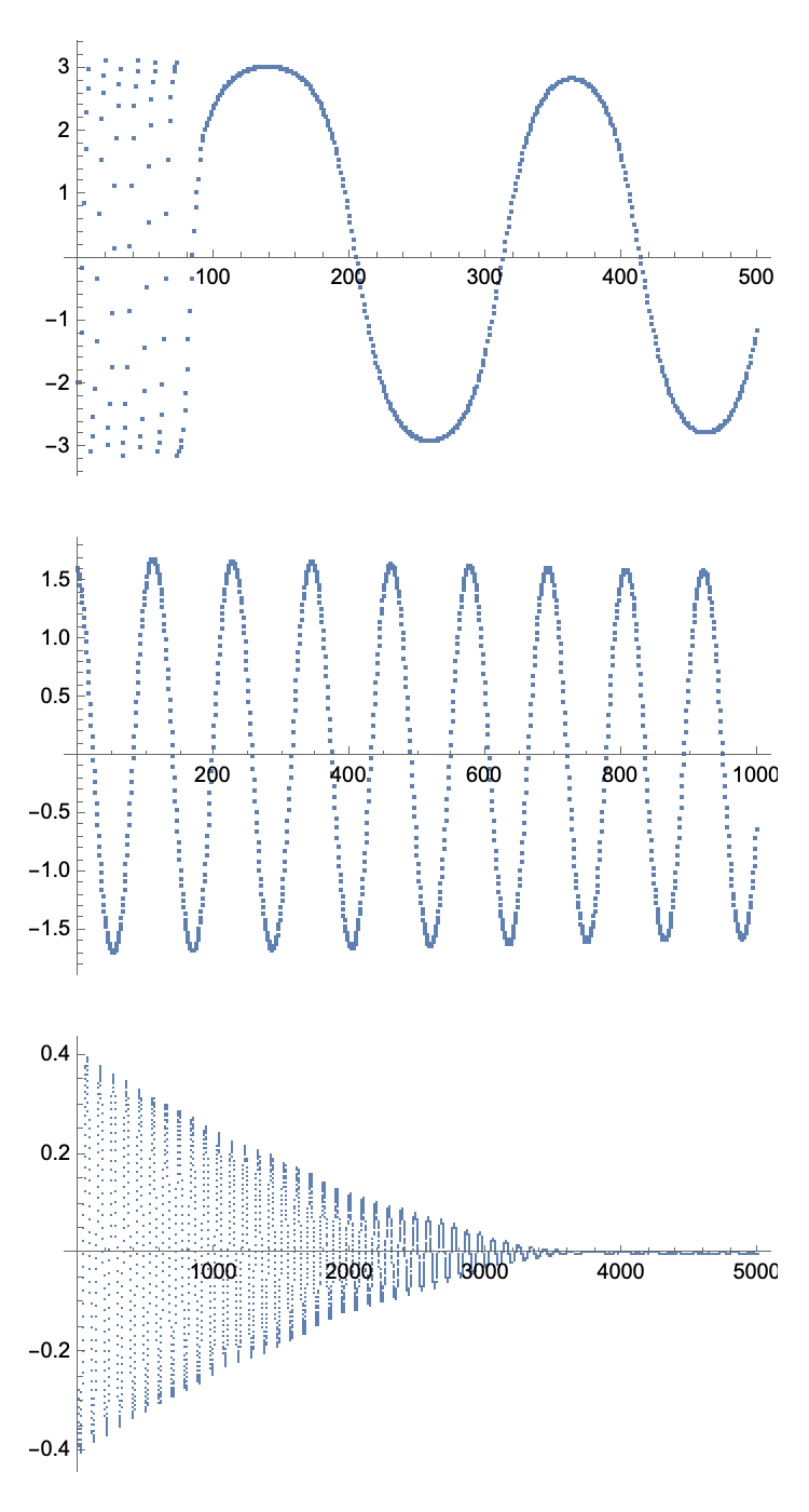
And then we can depict a few intervals of the data:

GraphicsColumn[ListPlot[#,
    ImageSize -> 400] & /@ {
   angleTimeseries[[1 ;; 500]],
   angleTimeseries[[5000 ;; 6000]],
   angleTimeseries[[-5000 ;; -1]]
   }]

Using Split we obtain half period intervals and convert them to Period-Energy data, again using a relatively expedient method (see note 22, page 70):

halfPeriodPartition = Rest[Most[SplitBy[angleTimeseries[[150 ;; -2500]], Sign]]];
wholePeriodPartition = Join @@@ Partition[halfPeriodPartition, 2];

periodEnergy = {
     Sin[Max[#]/2]^2, Length[#]
     } & /@ Abs[halfPeriodPartition];

FindFit[periodEnergy, t (2/Pi) EllipticK[x], {t}, {x}]

Out[] = {t -> 48.2605}

Using Length to get the periods is another expedient choice introducing significant error. The extracted value $2 \times 48 = 96$ is noticeably less than the value $104$ we obtained in the previous dissertation analysis. If the half-period frame count error is $1$, the period error is $\sigma = 2$, which puts the difference at $4\sigma$. This sounds suspicious, but also realize we are talking about a difference of only $3$ hundredths of a second. Let's not worry about this reproducibility issue too much right now, and loop back to it later if necessary.

Finally, we can check the plot by inspection to make sure the function agrees well with data:

Show[ListPlot[periodEnergy],
 Plot[2 48.26/Pi EllipticK[x], {x, 0, .99},
  PlotStyle -> Red], PlotRange -> All]

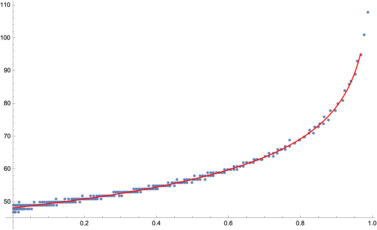
As far as shape is concerned, this data looks to agree quite nicely with the complete elliptic integral of the first kind. We could continue to extract one more parameter, anyone else want to try? A really nice model is also given in Figure 2.18, which shows up again in Chapter 4 on rigid body rotations. It's worth learning if you're studying for the Theoretical Minimum... Good Luck to you, it was too much for me!