Yes, with weighting function PDF[NormalDistribution[], #] & and data values around 80, the weights are values of the probability density function of the standard normal distribution around 80 standard deviations above the mean, so the weights are smaller (around 10^-1400) than the smallest possible machine number (which is about 10^-323). NormalDistribution[] refers to the standard normal distribution, which is the normal distribution with a mean of zero and a standard deviation of 1, so NormalDistribution is equivalent to NormalDistribution[0,1]. I don't know the limitations of the EstimatedDistribution function, but the error messages suggest that it is not designed to deal with weights that are that small. I'm not sure if that is what was intended here, but the following worked when I tried it:
sampleMean = Mean[wdAllFlat];

sampleStandardDeviation = StandardDeviation[wdAllFlat];

weightedData = WeightedData[wdAllFlat,
   PDF[NormalDistribution[sampleMean, sampleStandardDeviation], #] &];

EstimatedDistribution[weightedData, NormalDistribution[\[Mu], \[Sigma]]]
|
|
|
I have been experimenting with TTest and I am observing puzzling behavior. As the attached workbook shows, the SignificanceLevel option does not seem to change the p value for the sample dataset used in Lesson 27. The attached worksheet also shows experiments where the p value for a TTest with normally distributed data does not seem to decrease as the standard deviation of normally distributed data decreases. Perhaps I am making a mistake in how I am using TTest command.
 Attachments:
|
|
|
1) The significance level in a hypothesis test has no effect on the p-value. The significance level is the threshold for interpreting the p-value (deciding whether the p-value indicates a statistically significant departure from the null hypothesis). The SignificanceLevel option in the TTest function has an effect only if the interpretation is included in the output, as in:
In[]:= TTest[{1, 2, 3, 4, 5}, 1, {"PValue", "TestConclusion"}]

Out[701]= {0.0474207,
  The null hypothesis that the mean of the population is equal to 1 is rejected at the 5 percent level based on the T test.}

In[]:= TTest[{1, 2, 3, 4, 5}, 1, {"PValue", "TestConclusion"}, SignificanceLevel -> 0.01]

Out[702]= {0.0474207,
The null hypothesis that the mean of the population is equal to 1 is not rejected at the 1 percent level based on the T test.}
2) Unlike the sample that was used in the video, the mean of the sample generated by data1 = RandomVariate[NormalDistribution[1000, 0.254], 2500] is very close to 1000, and the sample size is 100 times bigger than the sample used in the video. Of those two differences, the most important difference here is that the sample mean is very close to 1000, which is the population mean under the null hypothesis. TTest[data1, 1000] will return a large p-value because the mean of the sample is (by construction) very close to 1000. Replacing 0.254 by 0.0254 or 0.00254 makes the population standard deviation smaller, but since the mean of the sample is still 1000, the p-values will be big. It is easier to see the effect of population standard deviation on the p-value by using samples from populations for which the mean is not equal the the mean under the null hypothesis, such as:
In[]:= data1 = RandomVariate[NormalDistribution[1001, 3], 10];
TTest[data1, 1000]

Out[]= 0.760372

In[]:= data2 = RandomVariate[NormalDistribution[1001, 1], 10];
TTest[data2, 1000]

Out[]= 0.0812006

In[]:= data3 = RandomVariate[NormalDistribution[1001, 0.5], 10];
TTest[data3, 1000]

Out[]= 0.0000260985
|
|
|
David, Thanks for your response. I will need to digest this carefully but I really appreciate your help. Joe Smith
|
|
|
Thanks again. Some additional experiments with data where the mean moves away from 1000 illustrate the interaction between PValue, the significance level, and the conclusion of the TTest with respect to rejection of the null hypothesis.
Attachments:
|
|
|
Please post the link to the course framework on this community site. The chat pane does not appear in the recording of the course so if I miss that lecture I won't see the link. Thanks!
|
|
|
Unfortunately the course framework is not ready for release yet. We are only sharing a beta version with our study group attendees. We can include the link in our reminder emails, so you can get to it, even if you miss the live session.
|
|
|
Hi; In using both functions NormalCI and MeanCI, I am getting some unexpected results - please see attached notebook. Thanks, Mitch Sandlin
Attachments:
|
|
|
In the notebook "11.NumericalSummariesOfData.nb" there are images of this kind:
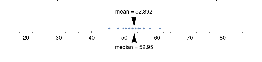 You animated these diagrams in the accompanying video and I wondered how you did it. Unfortunately, there are only pictures in the notebook (which makes sense, since you have explanations in the notebook that are "on the soundtrack" in the video). Even if it's a little off-topic, but: would you be so kind and share with us the code of this stunning animation?
|
|
|
Dear Mr. Withoff, Thank you very much for your answer. You are absolutely right, the code does distract a lot from the actual topic. There is also a separate course on the topic of "animations" here on WolframU. Still, thanks for sharing, I found your method of moving the five points or the single point via the join function (pts = ...) very enlightening. Also that you were able to assemble the final image with only "Epilog" was not something I would have expected.
|
|
|
Hi; I am interested in finding the value of "x" in a probability when I know the probability in which I am interested. Intuitively one would assume that the Solve function should produce the answer by simply solving for x - see below. However, Solve, SolveValue or Reduce does not return the desired results. In some situations, I know the probability in which I am interested but I do not know the value of x that gives that probability without a lot of trial and error, so I hope someone could point me in the right direction. Thanks,
Mitch Sandlin Solve[0.6 ==
Probability[x, x [Distributed] NormalDistribution[998, 202]], x]
|
|
|
Dear Mr. Sandlin: I am NO expert on Wolfram or Probability but the following may help you.
Attachments:
|
|
|
Hi Juan; Thanks so much. It was actually the InverseCDF function that performed the correct calculation. Mitch Sandlin
|
|
|
How to take the Quizzes and the Online Course Exam?
|
|
|
We will share links to quizzes and final exam during the DSG.
|
|
|
Show does not work properly in Mathematica 13.2.x. The overlay shown in the downloaded notebook 8.UsingHistogramData.nb fails to show the overlay!
Attachments:
|
|
|
Hi Marvin, The reason is that Show takes PlotRange from its first argument (Histogram) and you will notice that the second argument (ListLinePlot) has a very different PlotRange. Why??? Because, unexpectedly, MovingAverage performs a unit conversion from Celcius to Kelvin.
MovingAverage[{Quantity[22, "DegreesCelsius"], Quantity[24, "DegreesCelsius"]}, 2]
(* {Quantity[5923/20, "Kelvins"]} *)
To get the plots to overlay correctly, convert back to Celsius.
Show[Histogram[data, Automatic, "PDF"],
 ListLinePlot[
  Transpose[
   MapAt[UnitConvert[MovingAverage[#, 2], "DegreesCelcius"] &,
    HistogramList[data, Automatic, "PDF"], 1]], PlotMarkers -> All]]
This looks like a bug to me, or at least unexpected, undocumented (as far as I can tell) and can result in unexpected errors. You should report it to Wolfram Support.
|
|
|
Thank you, Abrita. Seeing the documentation is what I badly needed ! -Marv
|
|
|
Thank you very much for diagnosing the problem, Rohit! I got a response from support about the units on the x-axis not corresponding between the ListLinePlot and the graphic, and that was also not making sense to me at the time. Your response made it all very clear and, as you indicate, I do not think that this modification in implicit conversion was not documented in the prerelease documents I received for 3.2 or 3.3. It certainly is not compatible with the documentation and is possibly an easily corrected bug. I truly appreciate your persisting in analysis of this conundrum! I’ll re-report it to Support. -Marv Schaefer
|
|
|
Reminder that the statistics group starts Monday! Author @David Withoff will join us as we kickoff our latest Daily Study Group. A pre-release version of the interactive course framework will be shared with participants. Sign up here.
|
|
|
Reply to this discussion
in reply to
|