Here's a very ad hoc approach:
Jan = {2.09, 0.9, 317.4, 472.400, 417.79, 234.200, 325., 524.2, 49.59,
    114.7, 126.1, 136., 160.6, 203.2, 157.8, 0., 8., 23.5};

Feb = {0., 0., 0.5, 111.2, 155.700, 324.59, 152.5, 348.3, 222., 0.,
   0., 0., 0., 0., 24., 186., 118.3, 387.3};

Show[
 ListPlot[{{0.5, -250}, {4.5, 800}}, PlotRange -> {{0.5, 4.5}, {-250, 800}}, Frame -> True,
  FrameTicks -> {{Automatic, Automatic}, {{{1.5, "Jan"}, {3.5, "Feb"}}, None}}, PlotStyle -> White, Frame -> True],
 BoxWhiskerChart[{{}, Jan, {}, Feb}],
 DistributionChart[{Jan, {}, Feb, {}}, ChartElementFunction -> "SmoothDensity"],
 DistributionChart[{Jan, {}, Feb, {}}, ChartElementFunction -> "PointDensity",
  ChartStyle -> Directive[{GrayLevel[10, 10], Opacity[0.3], EdgeForm[]}]]
 ]
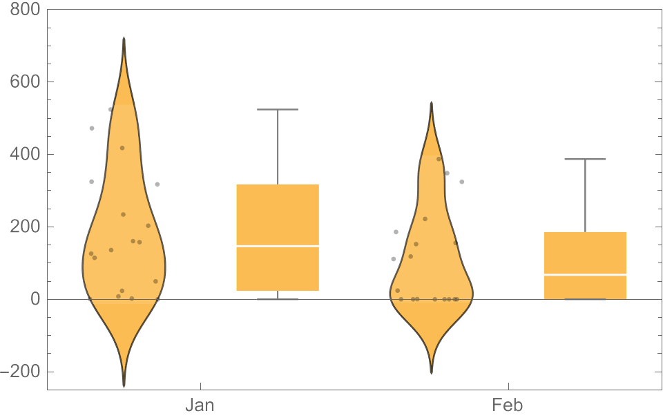
But your data is problematic for the available density plot in DistributionChart because those distributions are (likely) bounded by zero. Getting an appropriate density function for such cases would require the "Bounded" option in SmoothKernelDistribution.


