Firstly, in the program, X is a discrete expression about i (the specific analytical expression is in the For loop of the program), and the complete program is as follows:

{r = 22, l = 2 10^-1, c = 1 10^-4, vi = 24, initvalueil = 0, 
  initvaluevc = 0, tstart = 0, tend = 0.08, dt = 0.00006};
\[CapitalDelta]vi = 0;
n = (tend - tstart)/dt;
A = {{0, -1/l}, {1/c, -1/(r c)}};
G = Inverse[A];
B = {1/l, 0};
S1 = Inverse[DiagonalMatrix[{1, 1}] - dt*A + 1/2*dt*dt*A . A];
S2 = Inverse[DiagonalMatrix[{1, 1}] - dt*A];
STAR1 = S1 . G . (B*vi + G . B*\[CapitalDelta]vi/dt) - 
   G . (B*(vi + \[CapitalDelta]vi) + G . B*\[CapitalDelta]vi/dt);
STAR2 = S2 . G . (B*vi + G . B*\[CapitalDelta]vi/dt) - 
   G . (B*(vi + \[CapitalDelta]vi) + G . B*\[CapitalDelta]vi/dt);
X = Transpose[{{il, vc}}];
X0 = {0, 0};
errort = Table[tstart + dt*i, {i, 0, n}];
X1 = Table[{initvalueil, initvaluevc}, {i, 0, n}];
X2 = Table[{initvalueil, initvaluevc}, {i, 0, n}];
X = Table[{initvalueil, initvaluevc}, {i, 0, n}];
il = Table[0, {i, 0, n}];
vc = Table[0, {i, 0, n}];
For[i = 1, i < n + 1, i++,
  X[[i + 1]] = (MatrixPower[S1, i] - MatrixPower[S2, i]) . 
     X0 + (DiagonalMatrix[{1, 1}] . (DiagonalMatrix[{1, 1}] - 
         MatrixPower[S1, i]) . 
       Inverse[DiagonalMatrix[{1, 1}] - S1]) . 
     STAR1 - (DiagonalMatrix[{1, 1}] . (DiagonalMatrix[{1, 1}] - 
         MatrixPower[S2, i]) . 
       Inverse[DiagonalMatrix[{1, 1}] - S2]) . STAR2;
  il[[i + 1]] = X[[i + 1, 1]];
  vc[[i + 1]] = X[[i + 1, 2]];
  ];
p1 = Table[Transpose[{errort, il}], 1];
p2 = Table[Transpose[{errort, vc}], 1];
ListLinePlot[p1, AxesLabel -> {"s", "il[t]/A"}, 
 PlotLegends -> {"0.00006"}, PlotStyle -> {Red}, PlotRange -> All]
ListLinePlot[p2, AxesLabel -> {"s", "vc[t]/V"}, 
 PlotLegends -> {"0.00006"}, PlotStyle -> {Blue}, PlotRange -> All]

The curve obtained after executing the program is as follows: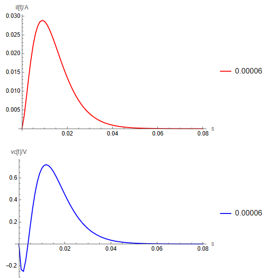

Next, I will replace i in the original X formula with t and dt, where dt is a constant and t is a variable. The complete program is as follows:

{r = 22, l = 2 10^-1, c = 1 10^-4, vi = 24, initvalueil = 0, 
  initvaluevc = 0, tstart = 0, tend = 0.08, dt = 0.00006};
\[CapitalDelta]vi = 0;
A = {{0, -1/l}, {1/c, -1/(r c)}};
G = Inverse[A];
B = {1/l, 0};
S1 = Inverse[DiagonalMatrix[{1, 1}] - dt*A + 1/2*dt*dt*A . A];
S2 = Inverse[DiagonalMatrix[{1, 1}] - dt*A];
STAR1 = S1 . G . (B*vi + G . B*\[CapitalDelta]vi/dt) - 
   G . (B*(vi + \[CapitalDelta]vi) + G . B*\[CapitalDelta]vi/dt);
STAR2 = S2 . G . (B*vi + G . B*\[CapitalDelta]vi/dt) - 
   G . (B*(vi + \[CapitalDelta]vi) + G . B*\[CapitalDelta]vi/dt);
X = Transpose[{{il, vc}}];
X0 = {0, 0};
X = ReplaceAll[(MatrixPower[S1, i] - MatrixPower[S2, i]) . 
     X0 + (DiagonalMatrix[{1, 1}] . (DiagonalMatrix[{1, 1}] - 
         MatrixPower[S1, i]) . 
       Inverse[DiagonalMatrix[{1, 1}] - S1]) . 
     STAR1 - (DiagonalMatrix[{1, 1}] . (DiagonalMatrix[{1, 1}] - 
         MatrixPower[S2, i]) . 
       Inverse[DiagonalMatrix[{1, 1}] - S2]) . STAR2, i -> t - dt];
il = X[[1]] // FullSimplify;
vc = X[[2]] // FullSimplify;

Plot[il, {t, tstart, tend}]
Plot[vc, {t, tstart, tend}]

The curve obtained after executing the program is as follows: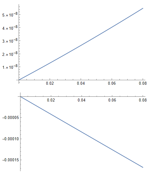

It is obvious that the curves are different. Where did I go wrong, or how did I convert a discrete equation to a continuous equation?