I have a CDF obtained with the code:

  dist = ProbabilityDistribution[{"CDF",     Exp[-a Exp[-x b] - c Exp[-x  d]]}, {x, 0, Infinity},   
          Assumptions -> {{0 < a < 10}, {0 < b < 1},   {0 < c < 10}, {0 < d <   1}}] 
  res = FindDistributionParameters[data,  dist, {{a, 3.8}, {b, 0.006}, {c, 0.08}, {d, 0.0002}}]

I can plot the confidence and prediction intervals following this demo for nonlinear pairs of data adjustment: http://demonstrations.wolfram.com/MeanAndSinglePredictionBandsForANonlinearModel/, and then http://rip94550.wordpress.com/2010/10/04/regression-1-%E2%80%93-two-kinds-of-prediction-bands/.

But for the custom CDF obtained with ProbabilityDistribution, I tried this:

Plot[{Func[x], bands90[x]}, {x, 0, 3000}, Filling -> {2 -> {1}}]

Without results.

Someone knows how to get the confidence and prediction bands in the case of CDF obtained with that function, as well as the ANOVA or the table that one can shows with ParamterTable (when fitting with NonlinearModelFit)?

As I see in some software is possible obtain more quality information for Nonlinear fitting that for distribution or custom distribution fitting, so I trying to construct my own code. To start getting the variance-covariance matrix I followed the code found here: Standard errors for maximum likelihood estimates in FindDistributionParameters And I elimitated the last part (Sqrt[Diagonal[cov]/len]]) as I also want to abtain the covariance matrix, so my code is:

covariance[data, dist, paramlist, mleRule] := Block[{len, infmat, cov}, len = Length[data]; (*compute negative of expected Fisher information*) infmat = -D[LogLikelihood[dist, data], {paramlist, 2}]/len /. mleRule; (invert to get asymptotic covariance) cov = Inverse[infmat]]

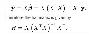
In this way I got the central part of the Hat matrix, (X^T X)^-1.

But somebody can verify if I'm in the right way? If so, I have to obtain X and X transpose, and then I have to add the variance s^2 to continue with the guide I found in http://rip94550.wordpress.com/2010/10/04/regression-1-%E2%80%93-two-kinds-of-prediction-bands/

Thanks you very much.