Message Boards

WOLFRAM COMMUNITY

1861 Views

4 Replies

5 Total Likes

View groups...

Follow this post

Share this post:

GROUPS:

How to extract Domain Segments and Coefficients of Interpolating Polynomials from InterpolatingFunc?

Július Weissenseiner

Posted 6 months ago

In Wolfram Mathematica, interpolated functions are often represented by the `InterpolatingFunction` object, which provides smoothed values of a function between given points (data). However, `InterpolatingFunction` hides internal details about how the interpolation is performed, including the domain segments where different interpolating polynomials are used, and the coefficients of these polynomials. I am interested in how to access this information, specifically the domain segments and coefficients of interpolating polynomials, to better understand or analyze how the interpolated function is constructed at the level of individual segments and polynomials.

POSTED BY: Július Weissenseiner

4 Replies

Sort By:

Robert Nachbar

Robert Nachbar, Wolfram Research Inc.

Posted 6 months ago

Have you looked at the functions in the "DifferentialEquations`InterpolatingFunctionAnatomy`" context. It's documented here.

POSTED BY: Robert Nachbar

Updating Name

Posted 6 months ago

Thanks for both approaches to solving this problem. If the InterpolatingFunction uses the Spline method, the individual intervals of the interpolating polynomials can really be read using InputForm[]. The approach of Mr. Schachner elegantly and skillfully creates individual interpolation polynomials from the input data. Thank you for your support. Regards, Július W.

POSTED BY: Updating Name

Henrik Schachner

Henrik Schachner, Radiation Therapy Center, Weilheim, Germany

Posted 6 months ago

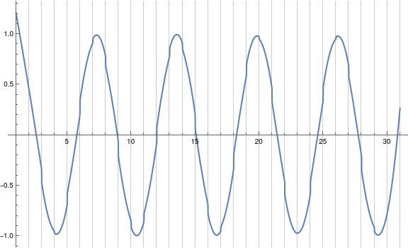
Július, here is an empirical approach: The idea is to consider the first derivative of the interpolation, because this way the composition of the whole curve seems to become more obvious: (* some test data: ) data = Table[N@Sin[x], {x, 0, 30}]; ( interpolated function - order '3' is default anyway: ) func = Interpolation[data, InterpolationOrder -> 3]; ( plotting its derivative: ) xrange = func[[1, 1]]; Plot @@ {func'[x], Flatten@{x, xrange}, GridLines -> {Range @@ xrange, None}, ImageSize -> Large} 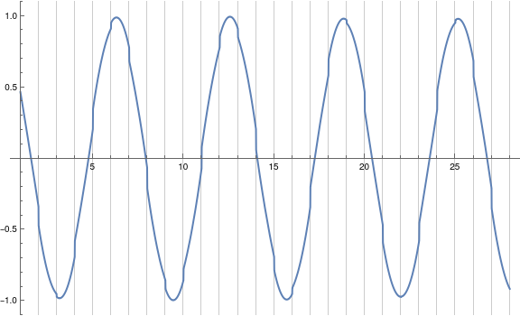You can mimic the very same* (apart from some shift in x) using interpolating polynomials in a piecewise manner: (* preparation for polynomial interpolation of order '3': ) ddata = Partition[MapIndexed[{First[#2 - 1], #1} &, data], 4, 1]; ( calculation of the polynomials: ) iPolygs = Expand@InterpolatingPolynomial[#, x] & /@ ddata; ( first derivative: ) diPolygs = D[#, x] & /@ iPolygs; xrange = Length[diPolygs]; ( piecewise plotting: *) Plot[diPolygs[[Round[x - .5]]], {x, 1, xrange}, GridLines -> {Range[xrange], None}, ImageSize -> Large] So - in a way that might be an answer to your question. (?) Regards -- Henrik

Július, here is an empirical approach:

The idea is to consider the first derivative of the interpolation, because this way the composition of the whole curve seems to become more obvious:

(* some test data: *)
data = Table[N@Sin[x], {x, 0, 30}];
(* interpolated function - order '3' is default anyway: *)
func = Interpolation[data, InterpolationOrder -> 3];
(* plotting its derivative: *)
xrange = func[[1, 1]]; Plot @@ {func'[x], Flatten@{x, xrange}, GridLines -> {Range @@ xrange, None}, ImageSize -> Large}

enter image description here

You can mimic the very same (apart from some shift in x) using interpolating polynomials in a piecewise manner:

(* preparation for polynomial interpolation of order '3': *)
ddata = Partition[MapIndexed[{First[#2 - 1], #1} &, data], 4, 1];
(* calculation of the polynomials: *)
iPolygs = Expand@InterpolatingPolynomial[#, x] & /@ ddata;
(* first derivative: *)
diPolygs = D[#, x] & /@ iPolygs;
xrange = Length[diPolygs];
(* piecewise plotting: *)
Plot[diPolygs[[Round[x - .5]]], {x, 1, xrange}, GridLines -> {Range[xrange], None}, ImageSize -> Large]

enter image description here