I want to calculate the table of confidence and prediction intervals for a custom Cumulative Distribution Function or CDF, and I am following the forums and articles aid.
My major cuestions that I repeat bellow are these:
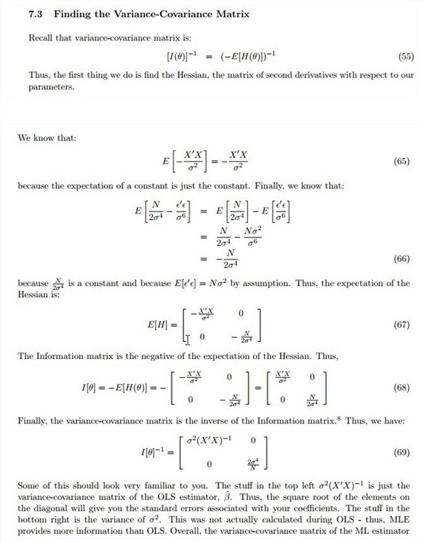
1.- I had to obtain the ACOV matrix and I use the inverse of the Information matrix for the Maximum Likelihood method (-inverse of the Fisher observed information matrix)number of data regarding the articles and forum revised. s this a correct way?
2.- When multiplying my vector or 1x1 matrix, as it is the partial derivate on only one variable, by the ACOV 4x4 matrix the software gives me another matrix, as if one multiplies a number times a matrix. Instead, we can obtain a simple number by adding three Zeros to the gradient vector, but I think that this is not correct. Then, what can we do if the number of columns in our vector is different that the number of rows in our ACOV matrix?.
First I want to share some about the theory:

This is the standard method that I want to apply in Mathematica, as we can find out in TableCurve 2 D or other software: 
I put here my DELTA METHOD TO OBTAIN THE VARIANCE OF A FUNCTION STEP BY STEP AND THEN THEIR CONFIDENCE AND PREDICTION INTERVALS OR BANDS: It seems that the key to carry out this method is in find the variance of the function that give us the prediction values) I find an example where I could test a part of the procces and I develop following:) Example http://www.montana.edu/rotella/502/DeltaExample.pdf in the case of female sex only.

VectorGrad = {1, -1, Li}; ACOVMatrix = {{0.04080, 0.0044646, -0.0054777}, {0.0044646082, 0.0438542, -0.0127939}, {-0.0054777, -0.0127939, 0.0486278733}}; (Applying the dot product to obtain the variance of the function) Var = VectorGrad.ACOVMatrix.VectorGrad;(Mathematica detect the same \n> vector to the right side and transposes it automatically)
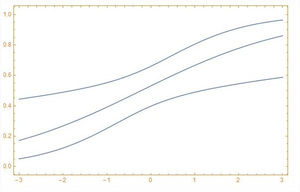
(The function to female rate,i.e., with sex=-1) fem = Exp[-0.416831 + 0.540171 + 0.564244 Li]/(1 + Exp[-0.416831 + 0.540171 + 0.564244 Li]); uc = -0.416831 + 0.540171 + 0.564244 Li + 1.96 Sqrt[Var]; uctran = Exp[uc]/(1 + Exp[uc]); ic = -0.416831 + 0.540171 + 0.564244 Li - 1.96 Sqrt[Var]; ictran = Exp[ic]/(1 + Exp[ic]); Show[Plot[uctran, {Li, -3, 3}], Plot[ictran, {Li, -3, 3}], Plot[fem, {Li, -3, 3}], PlotRange -> {{-3, 3}, {0, 1}}, AxesOrigin -> {-3, 0}, Frame -> True,
FrameStyle -> Directive[Orange, 12]]

HERE START MY CUSTOM CODE TO MY CUSTOM CDF with one variable (x)and four parameters (a,b,c,d). We find here two big differences that I resolved by myself and I have doubts to finish my block of code. 1.- I had to obtain the ACOV matrix and I use the inverse of the Information matrix for the Maximum Likelihood method (-inverse of the Fisher observed information matrix)number of data regarding the articles and forum revised. s this a correct way? 2.- When multiplying my vector or 1x1 matrix, as it is the partial derivate on only one variable, by the ACOV 4x4 matrix the software gives me another matrix, as if one multiplies a number times a matrix. Instead, we can obtain a simple number by adding three Zeros to the gradient vector, but I think that this is not correct. Then, what can we do if the number of columns in our vector is different that the number of rows in our ACOV matrix?.
- BUILD acov function. I used an snip of code found in http://mathematica.stackexchange.com/questions/6498/standard-errors-for-maximum-likelihood-estimates-in-finddistributionparameters but my doubt is: Why is divided by N or Lengh[data], is related to the Expectation function?. What this function do is to obtain the LogLikelihood function from the distribution and data, then execute the second derivative for the list of parameters and divides it by the length of the data. Finally it obtains the information matrix by remplacing the value of the parameters with the assignament symbol "/.".
acov[data, dist, paramlist, mleRule] := Block[{len, infmat, cov}, len = Length[data]; infmat = -D[LogLikelihood[dist, data], {paramlist, 2}]/len /. mleRule; cov = Inverse[infmat]];
- Define data and distribution.
data = {31, 46, 70, 87, 87, 93, 114, 128, 133, 134, 143, 155, 161, 161, 163, 177, 181, 207, 207, 226, 302, 315, 319, 347, 347, 362, 375, 377, 413, 440, 447, 461, 464, 511, 524, 556, 800, 860, 880, 954, 5200, 12000};
Distribution fitting.The distribution is devined as a CDF for a range x - infinity. To apply the MLE and obtain the paramters I gave initial values close to the final values that I knew from the fitting with another software.
dist = ProbabilityDistribution[{"CDF", Exp[-a Exp[-x b] - c Exp[-x d]]}, {x, 0, Infinity}, Assumptions -> {{0 < a < 10}, {0 < b < 1}, {0 < c < 10}, {0 < d < 1}}]; res = FindDistributionParameters[data, dist, {{a, 3.8}, {b, 0.006}, {c, 0.08}, {d, 0.0002}}]
The final parameters are : {a -> 3.7607209932409895, b -> 0.006209266160285994, c -> 0.0617315221225997, d -> 0.00014543291830692012} To obtain the ACOV we can use the acov function.
asincov = acov[data, dist, {a, b, c, d}, res];
- To calculate the gradient vector G' with respect to the only variable: x, i.e, partial derivative of G with respect x.
grad = D[Exp[-a Exp[-x b] - c Exp[-x d]], {x}] /. res;
- To obtain the variance - covariance parameters matrix (G' Transosed
Varian = grad.asincov.grad;
One can test the variance by pasing any value.
Varian /. {x -> 1};
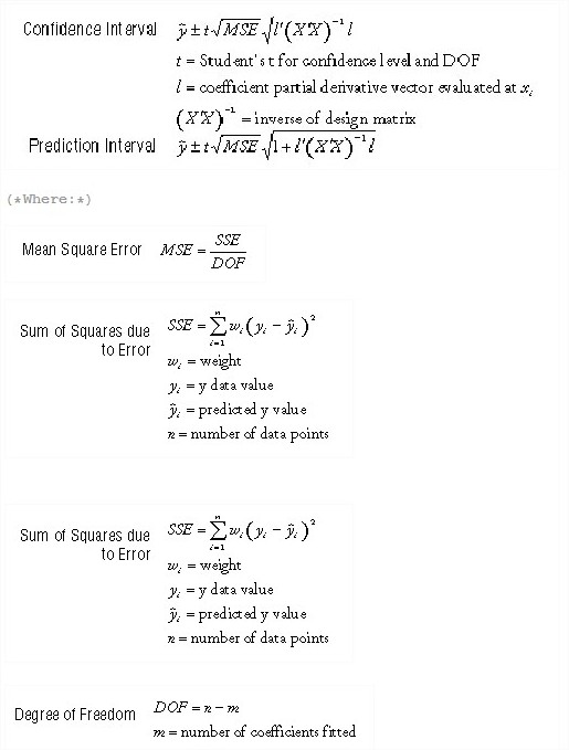
Following with the assesment of the confidence and prediction bands as we can see for example in the link http://stats.stackexchange.com/questions/15423/how-to-compute-prediction-bands-for-non-linear-regression, we have to evaluate the Critical t- Student value for confindence level, for example 95 %, and 42 - 4 = 38 degrees of freedom, in the case of 4 parameters and 42 data I sopose this is 38. That is, the critical t (N - 4, 0.05) = t(38, 0.05), is this correct?.
In Mathematica this is tantamount to the quantile for a t with 38 degree of fit and 0.95 confidence level:
Quantile[StudentTDistribution[41], 0.95];
Finally, we have to subtitute obtain sqrt (Varian) in the case of confidence intervals, or sqrt (1 + Varian) in the case of prediction intervals, as well as to assess the MSE to complete the formulas.
 Attachments: