While I'm now aware of the great functions Mathematica has for simulating stochastic processes on an unbounded domain, a common problem is a bounded domain with absorbing boundaries. In particular, once the process hits the boundary it stays there forever.

Is there an elegant and efficient way to include absorbing boundaries into simulations such as the following. That is, to have the boundaries (a,b) be absorbing?

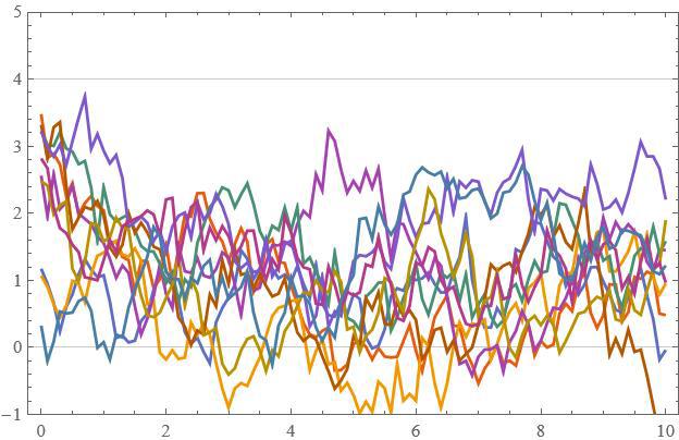
\[Mu] = 1;
\[Theta] = 1;
\[Sigma] = 1;

{a, b} = {0, 4};

numreps = 10;
Tmax = 10;
dt = .1;


paths = Table[
   RandomFunction[
    ItoProcess[\[DifferentialD]x[
        t] == \[Theta] (\[Mu] - 
          x[t])  \[DifferentialD]t + \[Sigma] \[DifferentialD]w[t], 
     x[t], {x, RandomReal[{a, b}]}, {t, 0}, 
     w \[Distributed] WienerProcess[]], {0, Tmax, dt}], {i, numreps}];

ListLinePlot[paths, PlotTheme -> "Scientific", 
 AspectRatio -> 1/GoldenRatio, 
 PlotRange -> {Automatic, {a - 1, b + 1}}, 
 GridLines -> {None, {a, b}}]