ABSTRACT (original article): Numerical tools for computation of ℘-functions, also known as Kleinian, or multiply periodic, are proposed. In this connection, computation of periods of the both first and second kinds is reconsidered. An analytical approach to constructing the Reimann surface of a plane algebraic curves of low gonalities is used. The approach is based on explicit radical solutions to quadratic, cubic, and quartic equations, which serve for hyperelliptic, trigonal, and tetragonal curves, respectively. The proposed analytical construction of the Riemann surface gives a full control over computation of the Abel image of any point on a curve. Therefore, computation of ℘-functions on given divisors can be done directly. An alternative computation with the help of the Jacobi inversion problem is used for verification. Hyperelliptic and trigonal curves are considered in detail, and illustrated by examples. CITATION (original article): Julia Bernatska, Computation of ℘-functions on plane algebraic curves, arXiv:2407.05632. https://doi.org/10.48550/arXiv.2407.05632

See first part here: Uniformization of a genus 4 hyperelliptic curve with arbitrary complex branch points

Introduction

In this discussion Example 3 from arXiv:2407.05632 is considered in detail. The present discussion can be considered as a continuation of discussion Uniformization of a genus 4 hyperelliptic curve with arbitrary complex branch points

A genus $g=3$ trigonal curve $\mathcal{C}$ in the canonical $(3,4)$-form, accurately defined below, serves as an example. A solution of the Jacobi inversion problem on this curve $\mathcal{C}$ is obtained from the system

$$ \mathcal{R}_6(x,y;u) = x^2 - y\, \wp_{1,1}(u) - x\, \wp_{1,2}(u) - \wp_{1,5}(u) $$

$$ \mathcal{R}_7(x,y;u) = 2 x y - y\, \big(\wp_{1,2}(u) - \wp_{1,1,1}(u)\big) \qquad\quad$$

$$\qquad\qquad\qquad\qquad\quad - x \big(\wp_{2,2}(u) - \wp_{1,1,2}(u) \big) - \big(\wp_{2,5}(u) - \wp_{1,1,5}(u)\big). $$

That is, given a point $u = (u_1, u_2, u_5) \in \mathrm{Jac}(\mathcal{C})$, which corresponds to a class of non-special divisors, one can find a reduced divisor $D$, which represents the class, such that $u=\mathcal{A}(D)$. This positive divisor $D$ of degree $g=3$ serves as a common divisor of zeros of the two entire rational (polynomial in $x$ and $y$) functions $\mathcal{R}_6$ and $\mathcal{R}_7$.

Multiply periodic $\wp$-functions, which arise in the definition of functions $\mathcal{R}_6$ and $\mathcal{R}_7$ are defined through the modular invariant entire function $\sigma$:

$\wp_{i,j}(u) = - \dfrac{\partial^2}{\partial u_i \partial u_j} \log \sigma(u),\qquad \wp_{i,j,k}(u) = - \dfrac{\partial^3}{\partial u_i \partial u_j \partial u_k} \log \sigma(u).$

In fact, uniformization is given by six functions which serve as coefficients of $\mathcal{R}_6$ and $\mathcal{R}_7$. Namely:

$$ \wp_{1,1}(u),\quad \wp_{1,2}(u),\quad \wp_{1,5}(u),$$ $$\wp_{1,2}(u)-\wp_{1,1,1}(u),\quad \wp_{2,2}(u)-\wp_{1,1,2}(u),\quad \wp_{2,5}(u) - \wp_{1,1,5}(u).$$ These six functions uniquely define a class of divisors linearly equivalent to $D$ such that $u=\mathcal{A}(D)$.

Trigonal curve

We consider the simplest trigonal curve in the canonical form, known as $(3,4)$-curve, namely $$ 0 = f(x,y) = -y^3 + y \mathcal{Q}(x) + \mathcal{P}(x) $$

$$ = -y^3 + y (\lambda_2 x^2 + \lambda_5 x + \lambda_{8}) + x^4 + \lambda_3 x^3 + \lambda_6 x^2 + \lambda_9 x + \lambda_{12}. $$

At every $x$ there exist three values of $y$, if the point is not a ramification point. We solve the equation of the curve for $y$ by the Cardano formula. Let $$\Delta(x) = \mathcal{P}(x) ^2 - \tfrac{4}{27} \mathcal{Q}(x) ^3$$ be the discriminant of the curve, and $$\upsilon(x) = \tfrac{1}{2} \big( \mathcal{P}(x) + \sqrt{\Delta(x)} \big).$$ Let $q_1, q_2, q_3$ denote three cubic roots of $\upsilon$: $$q_a (x) = \upsilon(x)^{1/3} \mathrm{e}^{2(a-1) \imath \pi/3},\quad a=1,2,3,$$ where $\upsilon^{1/3} $ is defined as follows $$\upsilon(x)^{1/3} = \left\{ \begin{array}{ll} |\upsilon(x)| \, \mathrm{e}^{(\imath/3) \arg \upsilon(x) } & \text{if } \arg \upsilon(x) \geqslant 0, \\ |\upsilon(x)| \, \mathrm{e}^{(\imath/3) \arg \upsilon(x) + \imath 2\pi / 3} & \text{if } \arg \upsilon(x) < 0; \end{array} \right. $$ and $\sqrt{\Delta}$ is defined as $$\sqrt{\Delta(x)} = \left\{ \begin{array}{ll} |\Delta(x)| \, \mathrm{e}^{(\imath/2) \arg \Delta(x) } & \text{if } \arg \Delta(x) \geqslant 0, \\ |\Delta(x)| \, \mathrm{e}^{(\imath/2) \arg \Delta(x) + \imath \pi } & \text{if } \arg \Delta(x) < 0. \end{array} \right. $$ Finally, $$y_a (x) = q_a(x) + \tfrac{1}{3} \mathcal{Q}(x)\, q_a^{-1},\quad a=1,2,3.$$

With the definition of $\upsilon^{1/3}$ introduced above, every $y_a$ has discontinuity over the contour $\Upsilon = \{x \mid \arg \upsilon(x)=0\}$, and the analytic continuation of $y_a$ is given by $y_b$, where $a \mapsto b$ according to a cyclic permutation $(123)$ or $(132)$.

The definition of $\sqrt{\Delta}$ introduces the contour $\Gamma = \{x \mid \arg \Delta(x)=0\}$, composed of segments $\Gamma_i$, each starts at $e_i$ and goes to infinity. Here $e_i$ is the $x$-coordinate of a branch point $B_i = (e_i,h_i)$ such that $h_i = y_a (e_i) = y_b (e_i )$. Then $y_a$ and $y_b$ have discontinuity over the contour $\Gamma$, and $y_b$ serves as the analytic continuation of $y_a$ on the other side of $\Gamma_i$, and vice versa.

Curve in Example 3

More precisely,

$$ f(x,y) = -y^3 + y (4 x^2 + 5 x + 11) + x^4 + 3 x^3 + 7 x^2 + 16 x + 9. $$ The curve has eight finite branch points: $$\begin{array}{llll} B_1 : & e_1 \approx -4.58931,& h_1 \approx -4.9092 & 2\text{-}3 \\ B_2 : & e_2 \approx -1.17922 - 0.934455 \imath,& h_2 \approx 1.60505 + 0.430221 \imath& 1\text{-}3 \\ B_3 : & e_3 \approx -1.17922 + 0.934455 \imath,& h_3 \approx 1.60505 - 0.430221 \imath &1\text{-}3 \\ B_4 : & e_4 \approx -0.431732 - 2.20256 \imath,& h_4 \approx 0.309255 - 1.83532 \imath& 2\text{-}3\\ B_5 : & e_5 \approx -0.431732 + 2.20256 \imath,& h_5 \approx 0.309255 + 1.83532 \imath& 1\text{-}2\\ B_6 : & e_6 \approx 0.499118 - 1.57527 \imath,& h_6 \approx -1.80047 + 1.31135 \imath& 1\text{-}2 \\ B_7 : & e_7 \approx 0.499118 + 1.57527 \imath,& h_7 \approx -1.80047 - 1.31135 \imath& 2\text{-}3 \\ B_8 : & e_8 \approx 0.812986,& h_8 \approx -2.42959& 2\text{-}3 \end{array} $$ In the right column the corresponding pair '$a\text{-}b$' is indicated, that is the pair of solutions $y_a$ and $y_b$ which coincide at $e_i$. On the figure below, the contour $\Upsilon$ is marked in green, and the direction in which $y_a$, $a=1,2,3$, connect according to the cyclic permutation $(123)$ is indicated by green arrows. The contour $\Gamma$ is marked in blue, and a pair '$a\text{-}b$' in blue indicates which solutions $y_a$ and $y_b$ connect along each segment of the contour. Some segments $\Gamma_i$ are intersected by the contour $\Upsilon$. At the points of such an intersection the pair '$a\text{-}b$' changes according to the cyclic permutation of $y_a$, $a=1,2,3$, along $\Upsilon$.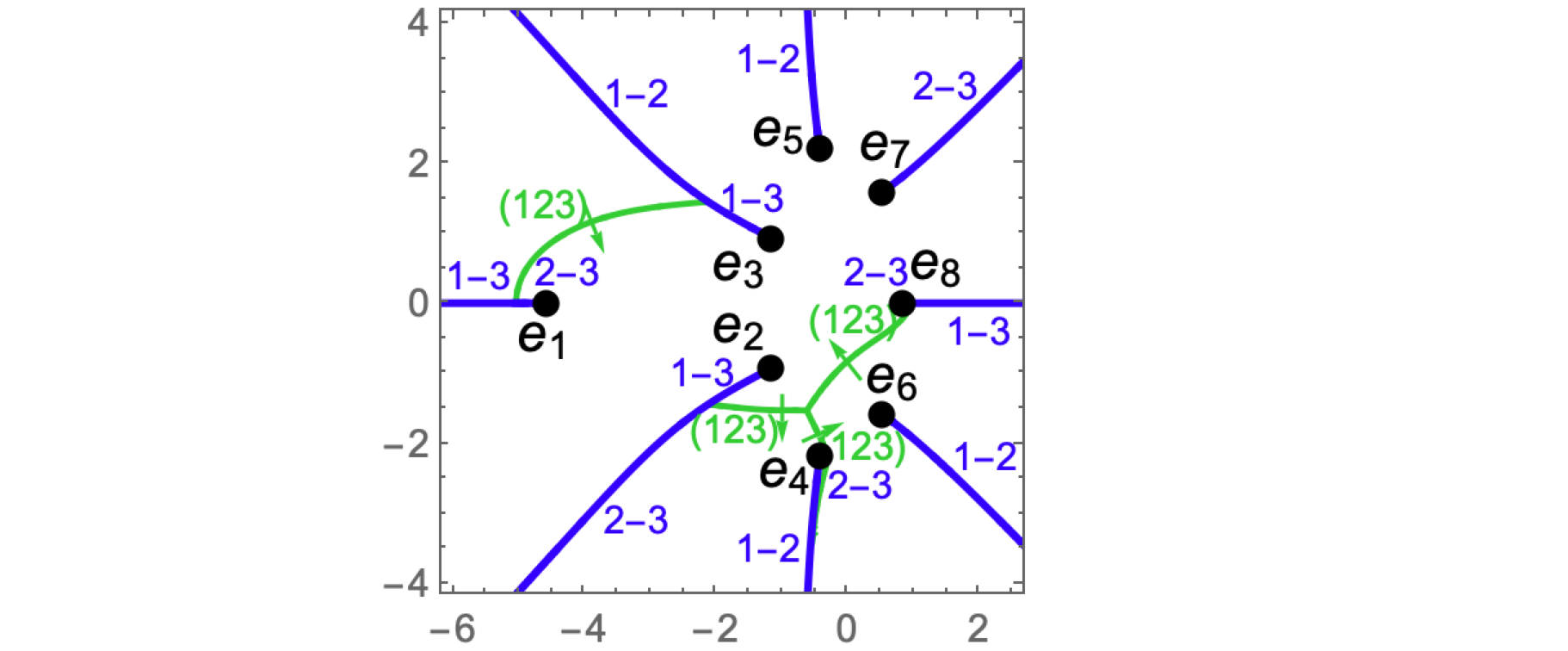

Riemann surface

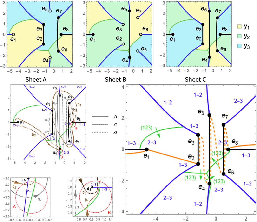
A trigonal curve has three sheets, which we denote Sheet A, Sheet B, and Sheet C. Two sheets join at every branch points, and all three sheets join at infinity.

The corresponding Riemann surface is obtained by making $g+1=4$ cuts along which two sheets are connected. Cuts are made between pairs of points:

• from $B_2$ to $B_3$ on sheets with solutions $y_1$ and $y_3$,
• from $B_4$ to $B_5$ on sheets with solutions $y_1$ and $y_2$ in the vicinity of $B_5$ which change consequently into the pair 1-3 and then 2-3 when approaching B4,
• from $B_6$ to $B_7$ on sheets with solutions $y_2$ and $y_3$ in the vicinity of $B_7$ which change into the pair 1-2 when approaching $B_6$.
• from $B_8$ to infinity, and then to $B_1$.

Further computations require the knowledge how $y_a$, $a=1,2,3$, change on each sheet. For this purpose, we draw a continuous path $\tilde{\gamma}$ on the $x$-plane from $-\infty$ to $\infty$ through all points $e_i$. The figure below shows this path, marked by orange. The path through all points $e_i$ is displayed by dashed lines between $e_2$ and $e_8$. The path $\tilde{\gamma}$ can be continuously deformed into a simpler path $\gamma$, displayed by solid lines. The both paths are polygonal, and go below points $e_i$, cuts are rounded counter-clockwise.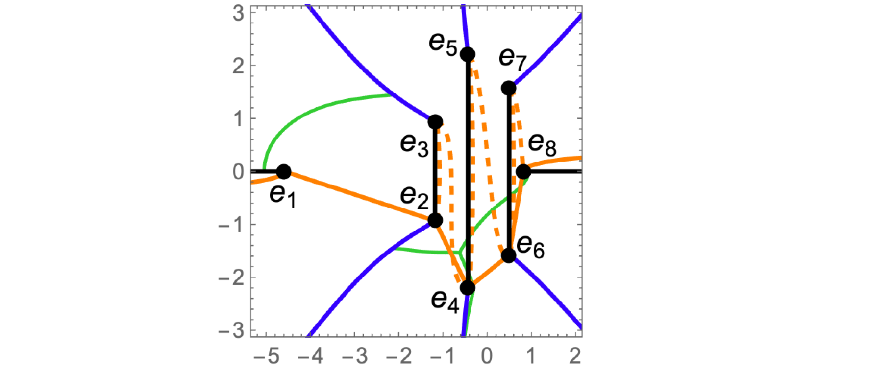

The path $\widetilde{\gamma}$ marks sheets as follows $$ \begin{array}{p{0.9cm}cccccccc p{0.9cm}} &\ \{a_{0-,1}, & a_{1,2}, & a_{2,3}, & a_{3,4}, & a_{4,5}, & a_{5,6}, & a_{6,7}, & a_{7,8}, & a_{8,0+} \} =\\ \text{Sheet A:} & \{\ \ 1, \ \ \ & 1, & 3, & 3\text{-}1, & 1\text{-}2\text{-}3,& 3\text{-}2,& 1\text{-}2, & 2, & 3\ \ \ \}, \\ &\ \{b_{0-,1}, & b_{1,2}, & b_{2,3}, & b_{3,4}, & b_{4,5}, & b_{5,6}, & b_{6,7}, & b_{7,8}, & b_{8,0+} \} =\\ \text{Sheet B:} & \{\ \ 2, \ \ \ & 2, & 2, & 2\text{-}3, & 2\text{-}3\text{-}1,& 1\text{-}3,& 3\text{-}1, & 1, & 1\ \ \ \}, \\ &\ \{c_{0-,1}, & c_{1,2}, & c_{2,3}, & c_{3,4}, & c_{4,5}, & c_{5,6}, & c_{6,7}, & c_{7,8}, & c_{8,0+} \} = \\ \text{Sheet C:} & \{\ \ 3, \ \ \ & 3, & 1, & 1\text{-}2, & 3\text{-}1\text{-}2,& 2\text{-}1,& 2\text{-}3, & 3, & 2\ \ \ \}. \end{array}$$ By $a_{i,j}$ the value $a$ of $y_a$ on segment $[e_i,e_j]$ is denoted on Sheet A, then by $b_{i,j}$ and $c_{i,j}$ similar values are denoted on Sheet B, and Sheet C, respectively. An expression of the form '$a$-$b$-$c$' means that over the corresponding segment the value $a_{i,j}$ in $y_{a_{i,j}}$ changes consequently from $a$ to $b$, then from $b$ to $c$.

Connection of solutions $y_1,y_2,y_3$ on each sheet is shown on the figure The $x$-plane is marked by three colors: yellow, light green, and sky blue, each shows where the areas of $y_1,y_2$, and $y_3$, correspondingly, are located. Every picture represents one sheet.

Note that all cuts can be reached on Sheet C, as well as all branch points.

Canonical homology basis

Let $\mathfrak{a}$-cycles encircle cuts between finite branch points counter-clockwise:

• $\mathfrak{a}_1$ encircles $[B_2,B_3]$
• $\mathfrak{a}_2$ encircles $[B_4,B_5]$
• $\mathfrak{a}_3$ encircles $[B_6,B_7]$

All $\mathfrak{a}$-cycles are located on Sheet C.

Let $\mathfrak{b}_k$-cycle emerges from the cut $[B_8,\infty)\cup (\infty,B_1]$ and enters the cut $[B_{2k},B_{2k+1}]$. Then $\mathfrak{b}_1$-cycle goes through Sheets C and A, $\mathfrak{b}_2$ through Sheets C and B, $\mathfrak{b}_3$ through Sheets C and A.

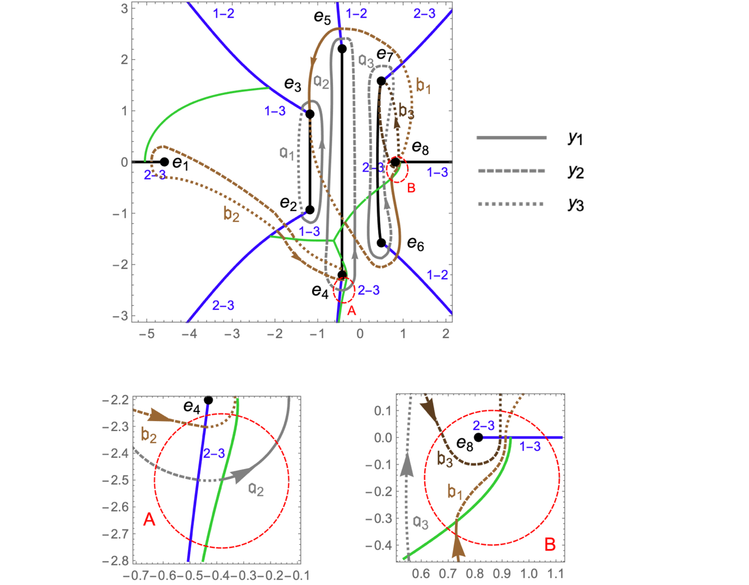On the figure, $\mathfrak{a}$-cycles are marked in grey, and $\mathfrak{b}$-cycles are marked in brown. Solid line stands for $y_1$, dashed for $y_2$, and dotted for $y_3$.

First and second kind differentials

A $(3,4)$-curve possesses the gap sequence $\{1,2,5\}$, and the first kind differentials have the form

$$ \mathrm{d} u = \begin{pmatrix} \mathrm{d} u_1 \\ \mathrm{d} u_2 \\ \mathrm{d} u_5 \end{pmatrix} = \begin{pmatrix} y \\ x \\ 1 \end{pmatrix} \frac{\mathrm{d} x}{-3 y^2+\mathcal{Q}(x)}. $$

Second kind differentials associated with the first ones on the curve are defined as follows $$ \mathrm{d} r = \begin{pmatrix} \mathrm{d} r_1 \\ \mathrm{d} r_2 \\ \mathrm{d} r_5 \end{pmatrix} = \begin{pmatrix} x^2 \\ 2 x y \\ \mathcal{R}_{5} \end{pmatrix} \frac{\mathrm{d} x}{-3 y^2+\mathcal{Q}(x)}, $$ $$\mathcal{R}_{5} = 5x^2 y + 3 \lambda_3 x y + \tfrac{2}{3}\lambda_2^2 x^2 + \lambda_6 y + \tfrac{2}{3} \lambda_2 \lambda_5 x.$$

First kind integrals

Let $\mathcal{A}^{[a]}_{i,j}$ denote the first kind integral between branch points $e_i$ and $e_j$ computed with $y = y_a(x)$:

$$\mathcal{A}^{[a]}_{i,j} = \int_{e_i}^{e_j} \mathrm{d} u^{[a]}.$$ Integrals are computed with the help of NIntegrate.

In order to verify, that the model of Riemann surface given above is constructed correctly, we compute first kind integrals along the path $\tilde{\gamma}$ on all Sheets. That is $$\mathcal{A}^{[n_{0,1}]}_{0,1} = \int_{-\infty-\imath \epsilon}^{e_1} \mathrm{d} u^{[n_{0,1}]}, \quad \mathcal{A}_{i,i+1}^{[n_{i,i+1}]} = \int_{e_{i}}^{e_{i+1}} \mathrm{d} u^{[n_{i,i+1}]},\ i=1,\dots,7,\quad \mathcal{A}^{[n_{8,0}]}_{8,0} = \int_{e_8}^{\infty+\imath \epsilon} \mathrm{d} u^{[n_{8,0}]},$$ where $n_{i,j}=a_{i,j}$, or $b_{i,j}$, or $c_{i,j}$, depending on the sheet.
The integrand of $\mathcal{A}_{i,j}^{[n_{i,j}]} $ is taken with $y =y_{ n_{i,j} }(x) $, and is a function of $x$. Note, that the path in $\mathcal{A}^{[n_{0,1}]}_{0,1}$ starts below the real axis, and the path in $\mathcal{A}^{[n_{8,0}]}_{8,0}$ ends above the real axis. This is essential for the relations presented below.

A lift of the continuous path to each sheet, closed by a semi-circle around infinity, is homotopic to zero, an so relations hold $$\mathcal{A}^{[n_{0,1}]}_{0,1} + \sum_{i=1}^{7} \mathcal{A}_{i,i+1}^{[n_{i,i+1}]} + \mathcal{A}^{[n_{8,0}]}_{8,0} = 0, \qquad n = a,\, b,\, c,$$ which serve for verification. In fact, a simpler path $\gamma$ is used. And relations acquire the form $$\mathcal{A}^{[1]}_{0,1} + \mathcal{A}^{[1]}_{1,2} + \mathcal{A}^{[3\text{-}1]}_{2,4} + \mathcal{A}^{[1\text{-}2]}_{4,6} + \mathcal{A}^{[1\text{-}2]}_{6,8} + \mathcal{A}^{[3]}_{8,0} = 0,\\ \mathcal{A}^{[2]}_{0,1} + \mathcal{A}^{[2]}_{1,2} + \mathcal{A}^{[2\text{-}3]}_{2,4} + \mathcal{A}^{[2\text{-}3]}_{4,6} + \mathcal{A}^{[3\text{-}1]}_{6,8} + \mathcal{A}^{[1]}_{8,0} = 0,\\ \mathcal{A}^{[3]}_{0,1} + \mathcal{A}^{[3]}_{1,2} + \mathcal{A}^{[1\text{-}2]}_{2,4} + \mathcal{A}^{[3\text{-}1]}_{4,6} + \mathcal{A}^{[2\text{-}3]}_{6,8} + \mathcal{A}^{[2]}_{8,0} = 0,$$ At the same time, another path homotopic to zero on each sheet exists, and so produces another set of relations: $$\mathcal{A}^{[3]}_{0,8} + \mathcal{A}^{[2]}_{8,7} + \mathcal{A}^{[3]}_{7,5} + \mathcal{A}^{[3]}_{5,3} + \mathcal{A}^{[1]}_{3,1} + \mathcal{A}^{[1]}_{1,0} = 0,\\ \mathcal{A}^{[2]}_{0,8} + \mathcal{A}^{[3]}_{8,7} + \mathcal{A}^{[2]}_{7,5} + \mathcal{A}^{[1]}_{5,3} + \mathcal{A}^{[3]}_{1,3} +\mathcal{A}^{[2]}_{1,0} = 0,\\ \mathcal{A}^{[1]}_{0,8} + \mathcal{A}^{[1]}_{8,7} + \mathcal{A}^{[1]}_{7,5} + \mathcal{A}^{[2]}_{5,3} + \mathcal{A}^{[2]}_{3,1} + \mathcal{A}^{[3]}_{1,0} = 0.$$ Evidently, $\mathcal{A}^{[n_{i,j}]}_{i,j} = - \mathcal{A}^{[n_{j,i}]}_{j,i}$, and $\mathcal{A}^{[a_{i,j}]}_{i,j}+\mathcal{A}^{[b_{i,j}]}_{i,j}+\mathcal{A}^{[c_{i,j}]}_{i,j} = 0$.

In fact, only integrals with one change of $y$-values are computed. The point where this change occurs on a line segment is found as a point of discontinuity of each $y_a$. Thus, integrals $\mathcal{A}^{[n_{2,4}]}_{2,4}$, $\mathcal{A}^{[n_{4,6}]}_{4,6}$, $\mathcal{A}^{[n_{6,7}]}_{6,7}$, $\mathcal{A}^{[n_{6,8}]}_{6,8}$ are computed with two different values of $y_a$. For example, on Sheet A $$\mathcal{A}^{[3\text{-}1]}_{2,4} = \int_{e_{2}}^{d} \mathrm{d} u^{[3]} + \int_{d}^{e_{4}} \mathrm{d} u^{[1]},$$ where $d$ denotes the point of intersection of the line segment $[e_2,e_4]$ with the contour $\Upsilon$.

Reducing the number of intersections with $\Upsilon$, we replace $\mathcal{A}^{[n_{4,5}]}_{4,5}$ with the sum $\mathcal{A}^{[n_{4,6}]}_{4,6}+\mathcal{A}^{[n_{6,5}]}_{6,5}$.

First kind periods

Periods are calculated according to the picture of homology cycles. Namely, $$\begin{array}{l} \omega_1 = \mathcal{A}^{[1]}_{2,3} + \mathcal{A}^{[3]}_{3,2},\\ \omega_2 = \mathcal{A}^{[3\text{-}1\text{-}2]}_{4,5} + \mathcal{A}^{[1\text{-}3\text{-}2]}_{5,4} = \mathcal{A}^{[3\text{-}1]}_{4,6} + \mathcal{A}^{[1\text{-}2]}_{6,5} + \mathcal{A}^{[1]}_{5,2} + \mathcal{A}^{[1\text{-}2]}_{2,4},\\ \omega_3 = \mathcal{A}^{[2\text{-}3]}_{6,7} + \mathcal{A}^{[2\text{-}1]}_{7,6},\\ \omega'_1 = \mathcal{A}^{[3]}_{8,7} + \mathcal{A}^{[2]}_{7,5} + \mathcal{A}^{[1]}_{5,3} + \mathcal{A}^{[3\text{-}2]}_{3,6} + \mathcal{A}^{[1\text{-}2]}_{6,8}, \\ \omega'_2 = \mathcal{A}^{[3]}_{1,2} + \mathcal{A}^{[1\text{-}2]}_{2,4} +\mathcal{A}^{[3\text{-}2]}_{4,2} + \mathcal{A}^{[2]}_{2,1}, \\ \omega'_3 = \mathcal{A}^{[3]}_{8,7} + \mathcal{A}^{[2]}_{7,8}. \end{array}$$ Here $\omega_k$ denotes the $k$-th column of $\mathfrak{a}$-period matrix $\omega$, and $\omega'_k$ denotes the $k$-th column of $\mathfrak{b}$-period matrix $\omega'$. These first kind period matrices are not normalized.

The Riemann period matrix is obtained by $$ \tau = \omega^{-1} \omega',$$ and is supposed to be a symmetric matrix with positive imaginary part. The latter serves for verification.

Second kind integrals and periods

A second kind integral $\mathcal{B}^{[a]}_{i,j} $ between $e_i$ and $e_j$ with $y = y_a(x) $ is computed by $$\mathcal{B}^{[a]}_{i,j} = \int_{e_i}^{e_j} \mathrm{d}r^{[a]}.$$ These integrals are used in computation of second kind periods, with respect to the same homology cycles. Namely, $$\begin{array}{l} \eta_1 = \mathcal{B}^{[1]}_{2,3} + \mathcal{B}^{[3]}_{3,2},\\ \eta_2 = \mathcal{B}^{[3\text{-}1\text{-}2]}_{4,5} + \mathcal{B}^{[1\text{-}3\text{-}2]}_{5,4} = \mathcal{B}^{[3\text{-}1]}_{4,6} + \mathcal{B}^{[1\text{-}2]}_{6,5} + \mathcal{B}^{[1]}_{5,2} + \mathcal{B}^{[1\text{-}2]}_{2,4},\\ \eta_3 = \mathcal{B}^{[2\text{-}3]}_{6,7} + \mathcal{B}^{[2\text{-}1]}_{7,6},\\ \eta'_1 = \mathcal{B}^{[3]}_{8,7} + \mathcal{B}^{[2]}_{7,5} + \mathcal{B}^{[1]}_{5,3} + \mathcal{B}^{[3\text{-}2]}_{3,6} + \mathcal{B}^{[1\text{-}2]}_{6,8}, \\ \eta'_2 = \mathcal{B}^{[3]}_{1,2} + \mathcal{B}^{[1\text{-}2]}_{2,4} +\mathcal{B}^{[3\text{-}2]}_{4,2} + \mathcal{B}^{[2]}_{2,1}, \\ \eta'_3 = \mathcal{B}^{[3]}_{8,7} + \mathcal{B}^{[2]}_{7,8}. \end{array}$$ Here $\eta_k$ denotes the $k$-th column of $\mathfrak{a}$-period matrix $\eta$, and $\eta'_k$ denotes the $k$-th column of $\mathfrak{b}$-period matrix $\eta'$. These second kind period matrices together with first kind period matrices $\omega$, $\omega'$ satisfy the Legendre relations, see [2] for more details.

We also compute the symmetric matrix $\varkappa$ required in the definition of $\sigma$-function: $$\varkappa = \eta \omega^{-1}.$$ Its symmetric property serves for verification.

Computation of $\wp$-functions

$\wp$-Functions are defined through $\sigma$-function, and the latter can be defined as a modification of the Riemann $\theta$-function: $$\sigma(u) = C \exp \big({-} \tfrac{1}{2} u^t \varkappa u \big) \theta [K] (\omega^{-1}u; \omega^{-1} \omega').$$ The characteristic $[K]$ of the vector of Riemann constants is found as a half-integer characteristic where $\theta$-function at $u=0$ has the maximal order of vanishing. This order is computed with respect to the Sato weight, which is $\mathrm{wgt}\, x = n = 3$, $\mathrm{wgt}\, y = s = 4$ on this curve. Also $\mathrm{wgt}\,\mathrm{d} u_i = -i$, and $\mathrm{wgt}\,\mathrm{d} r_i = i$, and numbers $i$ coincide with elements of the Weierstrass gap sequence.

It is known from [BEL1999], that on an $(n,s)$-curve $$\mathrm{wgt}\ \sigma(u) = - \frac{1}{24} (n^2-1)(s^2-1).$$ Let $\mathfrak{d} = - \mathrm{wgt}\ \sigma$, then $$ \frac{\partial^{\mathfrak{d}-1} \theta[K](\omega^{-1} u)}{\partial u_1^{\mathfrak{d}-1}} =0,\qquad \frac{\partial^{\mathfrak{d}} \theta[K](\omega^{-1} u)}{\partial u_1^{\mathfrak{d}}} \neq 0.$$

On the $(3,4)$-curve with the canonical homology basis defined above, we have

$$ [K]= \begin{pmatrix} 1 & 0 & 1\\ 0 & 1 & 1 \end{pmatrix}. $$

$\wp$-Functions can be computed in terms of $\theta$-function, see [2] for more details.

Example 3a

Let a divisor $D$ be composed of 3 points:

$$\begin{array}{ll} P_1 &= \big(e_3 - 0.5-0.5 \imath, y_1(e_3 - 0.5-0.5 \imath)\big) \\ &\approx (-1.679223 + 0.434455 \imath, 3.431176 - 0.582699 \imath), \\ P_2 &= \big(e_5 + 0.5-1.5 \imath, y_1(e_5 + 0.5-1.5 \imath)\big) \\ &\approx (0.068268 + 0.702564 \imath, 3.555003 + 0.889027 \imath),\\ P_3 &= \big(e_6 +1, y_1(e_6 +1)\big) \\ &\approx (1.499118 - 1.575269 \imath, -4.191263 + 1.058317 \imath). \end{array}$$

On the figure $x$-coordinates of the points are marked in orange, red, and magenta, as well as paths to them. 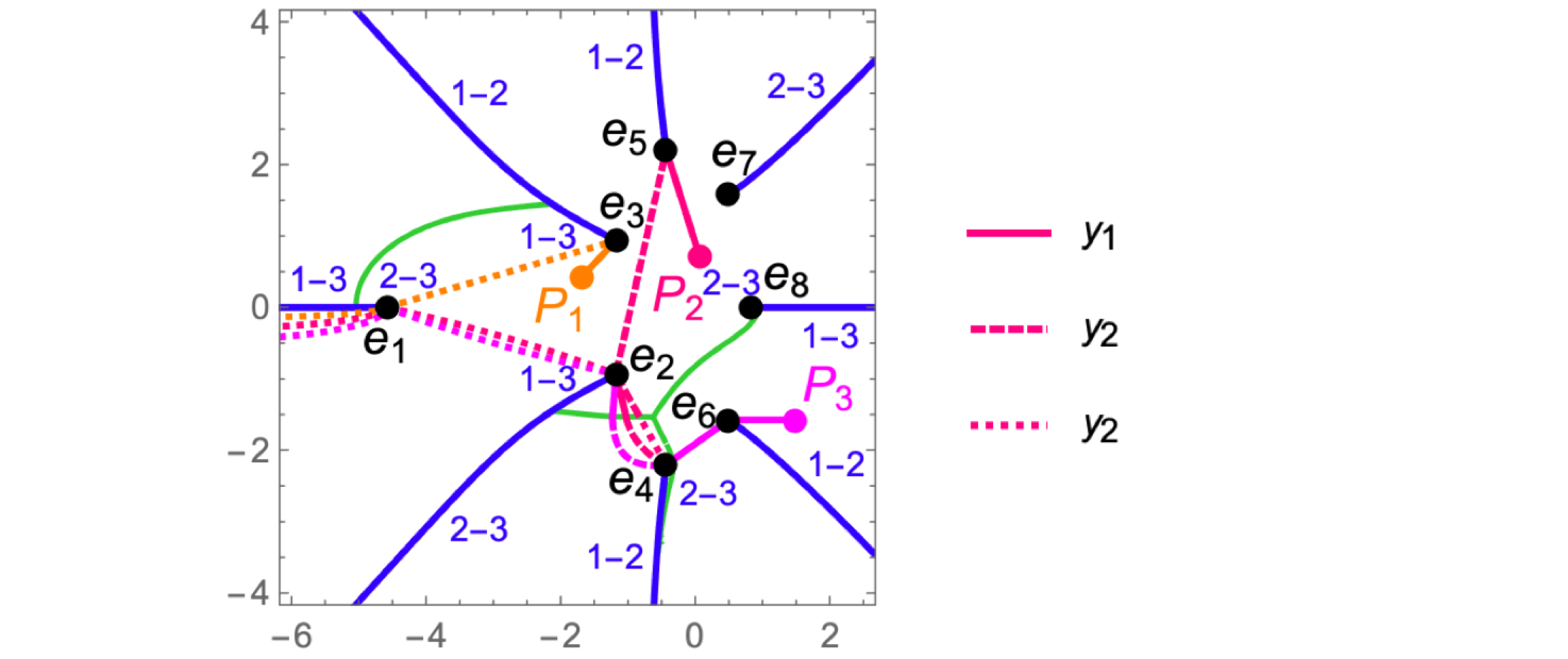The points $P_1$ and $P_3$ are located on Sheet A, and $P_2$ on Sheet B. A path to each point starts at $-\infty - \imath \epsilon$ on Sheet C. Below paths to each point are described in detail.

$P_1$ is close to the branch point $B_3$ on Sheet A. The path to $P_1$ which we choose goes from $-\infty$ below $B_1$ to $B_3$ on Sheet C, then enters the cut $[B_2,B_3]$ and emerges on Sheet A, and finally reaches $P_1$:

$$\mathcal{A}(P_1) = \mathcal{A}_{0-,1}^{[3]} + \mathcal{A}_{1,3}^{[3]} + \int_{e_3}^{P_1} \mathrm{d} u^{[1]}.$$

$P_2$ is close to $B_5$ on Sheet B. A path to $P_2$ goes on Sheet C from $-\infty$ below $B_1$ and $B_2$ to $B_4$. Here the path enters the cut $[B_4,B_5]$ and emerges on Sheet B, then goes to $(e_2,y_2(e_2))$ and to $B_5$, rounds $B_5$ from the above, and reaches $P_2$ on Sheet$\ $B:

$$\mathcal{A}(P_2) = \mathcal{A}_{0-,1}^{[3]} + \mathcal{A}_{1,2}^{[3]} + \mathcal{A}_{2,4}^{[1\text{-}2]} + \mathcal{A}_{4,2}^{[3\text{-}2]} + \mathcal{A}_{2,5}^{[2]} + \int_{e_5}^{P_2} \mathrm{d} u^{[1]}.$$

$P_3$ is close to $B_6$ on Sheet A. A path to $P_3$ goes on Sheet C from $-\infty$ below $B_1$, $B_2$ and $B_4$ to $B_6$. Then the path enters the cut $[B_6,B_7]$ and emerges on Sheet A, where it reaches $P_3$:

$$\mathcal{A}(P_3) = \mathcal{A}_{0-,1}^{[3]} + \mathcal{A}_{1,2}^{[3]} + \mathcal{A}_{2,4}^{[1\text{-}2]} + \mathcal{A}_{4,6}^{[3\text{-}1]} + \int_{e_6}^{P_3} \mathrm{d} u^{[1]}.$$ Here we use first kind integrals computed before. Integrals to points are computed with the help of NIntegrate.

Then the Abel image of $D$ is obtained by

$$\mathcal{A}(D) = \mathcal{A}(P_1) + \mathcal{A}(P_2) + \mathcal{A}(P_3).$$

The divisor $D$ is uniquely represented by the values of six $\wp$-functions at $u = \mathcal{A}(D)$:

$$ \wp_{1,1}(u),\quad \wp_{1,2}(u),\quad \wp_{1,5}(u),$$ $$\wp_{1,2}(u)-\wp_{1,1,1}(u),\quad \wp_{2,2}(u)-\wp_{1,1,2}(u),\quad \wp_{2,5}(u) - \wp_{1,1,5}(u),$$ which serve as coefficients of the two polynomial functions $\mathcal{R}_6$ and $\mathcal{R}_7$ defining a solution of the Jacobi inversion problem.

On the other hand, these two functions are computed from coordinates of the points of $D$:

$$\mathcal{R}_6 = \frac{\begin{vmatrix} 1 & x & y & x^2 \\ 1 & x_1 & y_1 & x_1^2 \\ 1 & x_2 & y_2 & x_2^2 \\ 1 & x_3 & y_3 & x_3^2 \end{vmatrix}} {\begin{vmatrix} 1 & x_1 & y_1 \\ 1 & x_2 & y_2 \\ 1 & x_3 & y_3 \end{vmatrix}},\qquad \mathcal{R}_7 = \frac{\begin{vmatrix} 1 & x & y & x y \\ 1 & x_1 & y_1 & x_1 y_1 \\ 1 & x_2 & y_2 & x_2 y_2 \\ 1 & x_3 & y_3 & x_3 y_3 \end{vmatrix}} {\begin{vmatrix} 1 & x_1 & y_1 \\ 1 & x_2 & y_2 \\ 1 & x_3 & y_3 \end{vmatrix}}.$$

The coefficients of $\mathcal{R}_6$ and $\mathcal{R}_7$ obtained in these two ways coincide with an accuracy of $10^{-11}$. This proves that the Abel images of the points are computed correctly.

Example 3b

Now we slightly modify the divisor $D$ by choosing different $y$-coordinates:

$$\begin{array}{ll} P_1 &= \big(e_3 - 0.5-0.5 \imath, y_2(e_3 - 0.5-0.5 \imath)\big) \\ &\approx (-1.679223 + 0.434455 \imath, -3.855009 + 0.446784 \imath), \\ P_2 &= \big(e_5 + 0.5-1.5 \imath, y_3(e_5 + 0.5-1.5 \imath)\big) \\ &\approx (0.068268 + 0.702564 \imath, -0.916997 - 0.935049 \imath),\\ P_3 &= \big(e_6 +1, y_3(e_6 +1)\big) \\ &\approx (1.499118 - 1.575269 \imath, 5.701625 - 3.318255 \imath). \end{array}$$

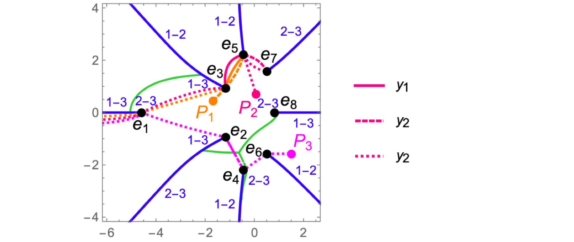
The points $P_1$ and $P_3$ are located on Sheet B, and $P_2$ on Sheet A. A path to every point starts at $-\infty - \imath \epsilon$ on Sheet C.

A path to $P_1$ goes above $B_1$ and $B_3$ to $B_5$ on Sheet C, then enters the cut $[B_4,B_5]$, emerges on Sheet B, goes to the point $(e_3, y_2(e_3))$, and reaches $P_1$:

$$\mathcal{A}(P_1) = \mathcal{A}_{0-,1}^{[3]} + \mathcal{A}_{1,3}^{[3]} + \mathcal{A}_{3,5}^{[1]} + \mathcal{A}_{5,3}^{[2]} + \int_{e_3}^{P_1} \mathrm{d} u^{[2]}.$$

A path to $P_2$ goes above $B_1$ $B_3$ and $B_5$ to $B_7$ on Sheet C, then enters the cut $[B_6,B_7]$, emerges on Sheet A, goes to $(e_5, y_3(e_5))$, and reaches $P_2$:

$$\mathcal{A}(P_2) = \mathcal{A}_{0-,1}^{[3]} + \mathcal{A}_{1,3}^{[3]} + \mathcal{A}_{3,5}^{[1]} + \mathcal{A}_{5,7}^{[2]} + \mathcal{A}_{7,5}^{[3]} + \int_{e_5}^{P_2} \mathrm{d} u^{[3]}.$$

A path to $P_3$ goes below $B_1$ and $B_2$ to $B_4$ on Sheet C, enters the cut $[B_4,B_5]$, emerges on Sheet B, goes to $(e_6, y_3 ( e_6 ))$ and reaches $P_3$:

$$\mathcal{A}(P_3) = \mathcal{A}_{0-,1}^{[3]} + \mathcal{A}_{1,2}^{[3]} + \mathcal{A}_{2,4}^{[1\text{-}2]} + \mathcal{A}_{4,6}^{[2\text{-}3]} + \int_{e_6}^{P_3} \mathrm{d} u^{[3]}.$$

Then we compute the six $\wp$-functions, which serve as coefficients of $\mathcal{R}_6$ and $\mathcal{R}_7$ and define the given divisor $D$ uniquely. By computing the functions $\mathcal{R}_6$ and $\mathcal{R}_7$ from coordinates of the points of $D$ we verify that the Abel images are found correctly.

References

[BEL1999] Buchstaber V. M., Enolskii V. Z., Leykin D. V., Rational analogs of abelian functions, Functional Analysis and Its Applications, 33:2 (1999) pp.83-94

Attachments:

AMap-C34-Exmpl3-Publ.nb