Group Abstract Group Abstract

Message Boards Message Boards

Modeling airflow past a car

Posted 3 months ago

POSTED BY: David Keith
16 Replies
Posted 10 days ago

This is only tangentially related so I won't be offended if you don't answer. I'm a new Mathematica user but I've done FEA in the past with CAD-based graphical FEA systems. It's a big change for me to be working the way it's done here. I have a question for either of you because I see your posts are relatively recent and I don't see a way to sort the forum by date so I can't easily find current discussions about a meshing problem I have. I'm trying to import a STEP file from Fusion360 and get it meshed in Wolfram, but I keep failing, even with a lot of help from the AI Chat feature. It also led me to a very simple STEP file from Wolfram's database and even that doesn't work.... I'm wondering if you have any experience with importing files for analysis, or if you know a better way for me to search the forum, or another source. The only filter I see is "Modeling" and there are still over 900 posts to look through with the search terms I've tried, many of them quite a few years old. I'd like to get a simple model of a block or beam from someone to import, if they have one that imports and meshes successfully. You guys seem like experienced forum users so I was hoping you might have an idea or two.

POSTED BY: Jeff Lastofka

Hi, From my understanding, Import["file.step"] mostly returns a Graphics3D object. Since STEP files are CAD representations, a better approach is to use OpenCascade functionality.

Needs["NDSolve`FEM`"]
Needs["OpenCascadeLink`"]

The general procedure is as follows

shapeIn = OpenCascadeShapeImport[path];

This produces an OpenCascade shape, which you can then convert into a mesh. For finite element analysis (FEM), the optimal workflow uses ElementMesh. You can create a boundary mesh as follows:

bmesh = OpenCascadeShapeSurfaceMeshToBoundaryMesh[shape];

and visualize it:

bmesh["Wireframe"["MeshElementStyle" -> FaceForm[Gray]]]

enter image description here

Note that this is a BoundaryMesh, so you may need to generate a full volumetric mesh for FEM analysis. You can do this with:

mesh = ToElementMesh[bmesh];
mesh["Wireframe"]

enter image description here

This mesh can then be used directly with NDSolve and other FEM procedures, as explained in the Structural Mechanics documentation.

As a closing note, the variable path used in OpenCascadeShapeImport[path] is a string that refers to the file you want to read. I tested this with several STEP files available online, and it generally works well. Alternatively, you can create and export your own model as follows:

reg = Cuboid[{0, 0, 0}, {10, 3, 1}];

This defines a region, which you can visualize as a graphic.

Graphics3D[reg]

enter image description here

You can then convert it into an OpenCascadeShape object and finally export it using:

path = FileNameJoin[{NotebookDirectory[], "test.step"}];
OpenCascadeShapeExport[path, shape];

For more details, see the OpenCascade documentation or this post (link) where I found some useful suggestions related to your question.

Hope this helps! Feel free to reach out if you encounter any issues.


Btw, the next step is to compute FEM:

vars = {{u[x, y, z], v[x, y, z], w[x, y, z]}, {x, y, z}};
pars = <|"YoungModulus" -> 10^9, "PoissonRatio" -> 0.33|>;
displ = NDSolveValue[{SolidMechanicsPDEComponent[vars, pars] == 
    SolidBoundaryLoadValue[x == lx, vars, 
     pars, <|"Force" -> {0, 0, -10000}|>], 
   SolidFixedCondition[x == 0, vars, pars]}, 
  vars[[1]], {x, y, z} \[Element] mesh]

For instance, left side fixed and right side with vertical load, the final deformation is:

VectorDisplacementPlot3D[displ, {x, y, z} \[Element] MeshRegion[mesh],
  PlotLegends -> Automatic]

enter image description here

Posted 8 days ago

Thank you for replying and I'm sorry I've hijacked this original discussion. I'll understand if you don't have time to continue here. No hard feelings. Not sure how to move it so I'll do at least one more reply here. Maybe you know of a better place.

I spent most of two days trying to get a working STEP (or other) import to mesh and analyze. I've used your example, MANY attempts with Notebook Assistant, some from ChatGPT - no success yet. Sometimes the mesh isn't right. Sometimes I get that seemingly OK and then the solver complains that I have more variables than equations.... I've gone back and forth with Notebook assistant checking things, and reading some of the documentation, but no luck. I used to do FEA at work sometimes. I've had training in and successfully used ANSYS, COMSOL, SDRC-Ideas, SolidWorks and Fusion360 for FEA over the years, and modeling a rectangular beam and doing a deflection and stress analysis would take a few minutes. I've spent an entire weekend trying to get one done in Mathematica and failed. I'm not giving up, but it seems an amazingly difficult and non-transparent process. (I don't want to model a simple geometry in Mathematica - I need to be able to import mechanical components from CAD - the simple rectangular beam is just to get a working procedure figured out - I've done the simple model within Mathematica and that works but it doesn't help me)

With a real FEA program like one of the above a person has a model to look at and can graphically apply constraints and make settings and see what's going on with the mesh, etc. In Mathematica there's a hidden room full of invisible commands and you have to know which commands to use in a proper order to guide the process. I expect I can eventually do this, but I need a working example to copy and learn from. It seems Notebook assistant almost works, but like ChatGPT it makes random mistakes along the way and the user has to point those out and have the A.I. reconsider and try again.

I'm in the evaluation period with the software. Not sure if I can call and ask for clues. I think they want us to use the forum and the Notebook assistant.

I think there were a couple of editing or pasting mistakes in the example you gave me but I think I worked around them OK.

bmesh["Wireframe"["MeshElementStyle" -> FaceForm[Gray]]]  

isn't really a command, for instance. I think all the Mathematica commands start with a capital letter. Perhaps just a detail, but I'm struggling to get an analysis to work so I'm still hoping to find at least one simple, complete, working example so I have a solid base to start from. I had Notebook Assistant find me an example STEP file from the Wolfram database and even that one failed.

Not giving up - just very disappointed so far. Thank you for trying to help. I suppose there must be some basic thing I'm assuming that's different from what Mathematica assumes. Like I don't understand how it thinks, so to speak. What I'm trying to do is very simple in other software, but those are prohibitively expensive and I'd like to learn Mathematica for this and other uses. I've been programming with it some and it's nice for that.

POSTED BY: Jeff Lastofka

Hi,

There’s no random copy-paste here, that’s exactly the sequence you need to load a STEP file correctly.

The only issue in the comment code was related to the input argument of:

bmesh = OpenCascadeShapeSurfaceMeshToBoundaryMesh[shapeIn];

It was mistakenly written as shape instead of shapeIn.

Also, note that bmesh is a variable, not a Mathematica function. You instantiate this variable as a BoundaryElementMesh object using the function above, which converts the OpenCascade shape into a boundary mesh representation.

Each BoundaryElementMesh object provides several built-in properties that you can easily access. For example, nodes:

bmesh["Coordinates"]

elements:

bmesh["BoundaryElements"]

or graphics:

bmesh["Wireframe"]

You can also add styling to the visualization, for example:

bmesh["Wireframe"["MeshElementStyle" -> FaceForm[Gray]]]

Or in general:

bmesh["Properties"]

In the Wolfram Language, some symbolic objects, such as BoundaryElementMesh, ElementMesh, or Dataset, act as data containers rather than pure functions. The expression bmesh["Wireframe"] means: ask the object bmesh to return its “Wireframe” representation.

This design makes it easy to access multiple views or derived data from the same object without defining separate functions. In other words, "property" acts like a method or query applied to the object, not a global function call. For more information on the mesh["Properties"] read Element Mesh Generation and Element Mesh Visualization documentation pages.


Coming back to your problem, I understand that you mainly work with FEM software that provides a graphical user interface (GUI). However, there are many other FEM tools that rely primarily on a command-line interface.

The strength of Mathematica lies in its symbolic representation combined with its dynamic visualization capabilities. To correctly describe a mechanical (structural) problem, you must specify the boundary conditions. This can easily be done using dedicated functions, see the reference Solid Mechanics - Boundary Conditions for detailed guidance.

The key idea is to express the locations where you want to apply the boundary conditions (which you would normally click on in a GUI) as logical conditions. For example,

x == 0

applies the boundary condition to all nodes where x is 0.

These boundary-condition functions often require two additional arguments:

  • vars, the list of dependent variables in your PDE system
  • pars, association of parameters, such as material properties.

You also need to specify the type of condition, for instance:

SolidBoundaryLoadValue[ x == lx, vars, pars, <|"Force" -> {0, 0, -10000}|>]

This defines a force-type boundary condition, of magnitude -10000, along the z, acting on all nodes where x == lx. The function returns a symbolic representation, not a numerical result, it’s part of the system definition you’ll later pass to NDSolve.

{ op == bv, bcs }

where:

  • op is the operator obtained from the main structural equations,
  • bc is the boundary load (or zero if the system is unloaded),
  • bcs is the list of boundary conditions (fixed, sliding, etc.).

The operator is defined as:

op = SolidMechanicsPDEComponent[vars, pars]

which represents the governing equation linking stress and strain. See the reference Solid Mechanics monograph for a full derivation, but you don't need all the mathematical details now.

Once you have op, bv, and bcs, you can use:

pde = {op == bv, bc1};
displ = NDSolveValue[pde, vars[[1]], {x, y, z} \[Element] mesh]

to obtain the solution for your FEM model. See te attached notebook.

I strongly recommend reading the Structural Mechanics monograph and reproducing a few examples to become familiar with the overall workflow. I’m also attaching the complete notebook instead of splitting the code so you can reproduce the process directly. By the way, which version of Mathematica are you using? If possible, try running it on a recent version, it may help avoid compatibility issues. Otherwise, feel free to reach out with details about your specific application, and we can help you troubleshoot your case.


Posted 7 days ago

Thank you VERY much for continuing to help. I had found that little typo and fixed it - not just trying a few things here and there - have put a lot of time into this. I've got 10 days left in the trial period and I can see I won't likely get this sorted out by then so I plan to just subscribe and keep going because I'm encouraged that you were able to import an actual mechanical part and analyze it. Clearly the process can work.

However, the notebook you sent fails for me early, on the OpenCascade import step:

with

CreateManagedLibraryExpression: The name OpenCascadeShapeManager is not registered as a library expression manager.

and

OpenCascadeShapeImport::file: An error was found loading stp file, /Users/jefflastofka/Library/Mobile Documents/com~apple~CloudDocs/Programming/Wofram Mathematica/WallHook_30mm.stp.

and

$Failed

but I'll bet I need to fix the first one first. I hadn't seen this error before, but going back and checking some previous Notebook attempts I found NUL returns that were previously hidden because of semicolons at the ends of statements it seems. Now that I'm learning more about the software I'm getting better at poking around and looking for those things.

(Wolfram could have an Import3DObject command that brings in a file and performs a list of standard tests to verify it's suitable for analysis, rather than relying on the user to remember a list of things to check, or deal with failures later.)

I searched for compatilibilty in the documentatin and on Wolfram's site and couldn't find it, so I used their Chat Agent to find the link. It doesn't help much, going up to OS15 for the Mac and I'm on the latest 26.0.1 with an M4 chipped Mac mini with 24GB RAM and I ran the Wolfram Benchmark tests and got a system score of 2.35 and no errors flagged, so I guess things are fine there. And I have Wolfram 14.3 so all is likely good. Maybe I've run into a bug they didn't know about. Maybe a software reinstall or something but I've never had to do that with any software I can think of.

I'm learning quite a bit about talking to the Wolfram software from your notes and I'll be reading some more in the links you sent. I'm not giving up. It's just going to take a lot more time and effort than I expected. It's still very disappointing I haven't found a simple working Notebook I can study and work from. Perhaps if I sort out this OpenCascade issue I'll be there with the one you kindly sent.

I had already noticed the boundary constraint application techniques and they're fine for research purposes or contrived academic problems with nice boundaries. However, I can imagine a pressure vessel, for instance, with a complicated internal shape and trying to apply a pressure - seems to be a nightmare to specify but I'll ignore that for now. I need to get something simple working first. I feel like I might be getting close, thanks to you.

The notebook assistant, just like ChatGPT, is simultaneously very helpful and annoyingly (dangerously) wrong, often within the same reply, and then it corrects itself (somewhat, anyway) when you challenge it. Another new tool to learn to work with :-)

POSTED BY: Jeff Lastofka
Posted 4 days ago

Update for you. Your notebook works fine for me now. I went back and forth with tech support at Wolfram and there's an incompatibility with the new Mac OS. They got me a new folder of files to install and things are MUCH better. Several examples I'd been trying now work. Phew - now I can start to learn from them. It's been quite a struggle. Thanks for the assistance.

POSTED BY: Jeff Lastofka

Hi Jeff, Glad to hear that! Another suggestion would be to try opening the app on the new Mac using Rosetta (right-click → Get Info → make sure “Open using Rosetta” is checked). Also, please make sure to report any technical issues you encounter, it really helps us improve the software.

Posted 4 days ago

Oh, tech support knows, they found the issue for me and gave me the folder of new files to fix it. I'm going to buy the software and A.I. assistant in a couple days. Thanks !

POSTED BY: Jeff Lastofka
Posted 7 days ago

Hi Jeff.

I wanted to share this blog, which you may find useful, as it introduces a general workflow for solving PDEs in the Wolfram Language, using a simple model of boiling an egg: https://blog.wolfram.com/2025/09/15/how-long-to-boil-an-egg-fem-modeling-with-wolfram-language/

Also, if you are not too familiar with the concepts of the Wolfram Language in general, it might be worth taking a look at this free course: https://www.wolfram.com/wolfram-u/courses/wolfram-language/an-elementary-introduction-to-the-wolfram-language/. Or this fast introduction: https://www.wolfram.com/language/fast-introduction-for-programmers/en/.

Cheers, Ricardo.

POSTED BY: Ricardo Lopez
Posted 6 days ago

Thank you for the ideas. I'd looked through some of that already but will be going back over it now that I'm serious about subscribing and using the language. I had also contacted tech support and they got back to me with a Notebook file that creates a solid, writes it out as a STEP and reads it back in, but that fails on my machine, too, with different error messages than I've seen before. Something about commands being missing. I think there could be a problem with the latest MacOS and latest Mathematica perhaps? Anyway, I'll see what support replies. Meanwhile I'll go back to more general programming, which was working nicely for me, and I'll re-attempt the STEP things later.

POSTED BY: Jeff Lastofka
Posted 4 days ago

I don't know if you saw my other reply but the problem turned out to be incompatibility with the new Mac OS. I got new files from tech support and things work now.

POSTED BY: Jeff Lastofka
Posted 3 months ago

Thank you, Alessandro. I appreciate the help.

The first step is to obtain a better mesh, as you point out. (I should have seen that!) I have tried to refine the mesh by using

mesh = ToElementMesh[\[CapitalOmega], MaxCellMeasure -> .1, 
   "MaxBoundaryCellMeasure" -> .001];
mesh["Wireframe"]

This works for the example in the documentation using a Disk, but for my RegionDifference (which has Head Polygon) the MaxBoundaryCell option has no effect. I have also tried first creating a BoundaryMesh of Omega, then handing that to ToElementMesh. That also has no effect. I could just use a smaller MaxCellMeasure, but that creates smaller cells even where they are likely not needed. Perhaps you could say more about the process of applying a finer discretization to the car rectangle. I have read all the guide on meshing, but still can't figure out how to control a mesh in that manner.

In another tool I have used there is a tree structure that allows a mesh to be built up under user control, including the separate construction of meshes on boundaries. It could produce a mesh like that below. Is there a capability in Mathematica that can get similar results? enter image description here

POSTED BY: David Keith

I realize this isn’t a trivial issue, mainly due to how ResourceFunction["RoundedPolygon"] works.

While with the Rectangle[] you can use "MaxBoundaryCellMeausure" to set you discretization:

bMeshRec = ToBoundaryMesh[rec, "MaxBoundaryCellMeasure" -> carLength/2];
Length[bMeshRec["Coordinates"]]
52

or by dividing carLength by 10:

bMeshRec = ToBoundaryMesh[rec, "MaxBoundaryCellMeasure" -> carLength/10];
Length[bMeshRec["Coordinates"]]
260

The issue is that ResourceFunction["RoundedPolygon"] returns a predefined, discretized geometry, so ToBoundaryMesh ends up using those fixed coordinates. That’s why it appears not to work properly with ToElementMesh. However, here’s a workaround I found, it’s a bit tricky, but it not only solves the problem, it also gives better insight into how these functions behave.

Solution A is to build the car geometry using a combination of pure Region functions, such as Disk[] and Rectangle[], which gives you more control over the cells size once you pass it to ToElementMesh.

Solution B is to modify the existing boundary mesh to match your desired resolution. For example, you can create two separate BoundaryElementMesh objects with your custom discretization, then join them together and fill in the interior elements afterward.

External rectangle: this is straightforward, as shown earlier, you can set your desired "MaxBoundaryCellMeasure" to control the discretization. Note that you can (and will need to for the next step) extract both the coordinates and the connectivity. Since this is a boundary mesh, the connectivity simply defines line elements between consecutive points.

rec = Rectangle[{0, 0}, {recLength, recHeight}];
bMeshRec = ToBoundaryMesh[rec, "MaxBoundaryCellMeasure" -> carLength/10];
coordsRec = bMeshRec["Coordinates"];
(* [[1,1]] take the first, in this case the singile one, from the list, and then all the connectivity inside LineElement *)
connRec = bMeshRec["BoundaryElements"][[1, 1]];

You can apply the same approach to the car geometry, but keep in mind that "MaxBoundaryCellMeasure" has no effect in this case. My solution is to manually insert additional points between each pair of existing points, so that each segment is discretized according to your desired resolution. Note that the spacing between points is not uniform, corner segments are shorter than the longer sides (see figure).

bMeshCar = ToBoundaryMesh[car, "MaxBoundaryCellMeasure" -> 1];
coordsCar = bMeshCar["Coordinates"];
connCar = bMeshCar["BoundaryElements"][[1, 1]];

To visualize the points distance:

Graphics[{Point[coordsCar],
  {If[Norm[Differences[coordsCar[[#]]]] < carHeight, Red, Blue], 
     Line[coordsCar[[#]]]} & /@ connCar
  }, PlotRange -> {{carx, carx + carLength/2}, {cary + carHeight/2, cary + carHeight}}]

enter image description here

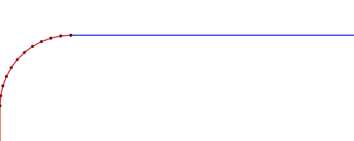
So you’ll need to compute the ideal number of subdivisions for each segment individually. Note that I used Max[ xxx , 2] in the computation to avoid division by zero during points placement, for smaller spacing you won't need it.

Once you understand the logic, you can easily tweak it to suit your needs. And you can do it with:

finerCoords = {};
spacing = carLength/50;
sortingIdx = FindShortestTour[coordsCar][[2]];
sortedCoords = coordsCar[[sortingIdx]];
Do[
  pt0 = sortedCoords[[i]];
  pt1 = sortedCoords[[i + 1]];
  n = Max[Ceiling[Norm[pt1 - pt0]/spacing], 2];
  pts = Table[pt0 + k ( pt1 - pt0)/(n - 1), {k, 0, n - 1}];
  AppendTo[finerCoords, #] & /@ pts;
  , {i, 1, Length[sortedCoords] - 1}];
finerCoordsLen = Length[finerCoords];
newConnectivity = Join[Table[{i, i + 1}, {i, finerCoordsLen - 1}], {{finerCoordsLen, 1}}];

And then you need to join the two boundary mesh information togheter:

updatedConnectivity = newConnectivity + Length[coordsRec];
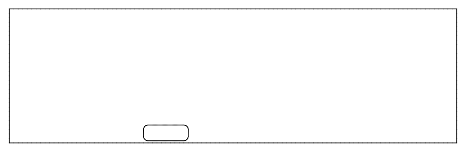
bmesh = ToBoundaryMesh["Coordinates" -> Join[coordsRec,  "BoundaryElements" ->{LineElement[connRec], LineElement[updatedConnectivity]}];
bmesh["Wireframe"]

enter image description here

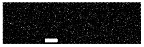
At this point, you can mesh the interior region and specify "MaxCellMeasure" to control the element size inside. Just keep in mind that this setting will not affect the boundary discretization. You need to specifiy also the Hole coordinates, you can simply use the center of the car.

mesh = ToElementMesh[bmesh, "RegionHoles" -> Mean[coordsCar], "MaxCellMeasure" -> .1];
mesh["Wireframe"];

enter image description here

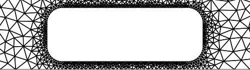
Note that although the result may look quite similar at first glance, if you zoom in on the bottom side of the car, you’ll see that the discretization is now much finer.

Show[mesh["Wireframe"], PlotRange -> {{0.9 carx, 1.1 carx + carLength}, {0, cary + carHeight}}]

enter image description here

You can adjust the spacing variable and the boundary discretization as needed to control the resolution more precisely.

Posted 3 months ago

Thank you very much for your help, Alessandro. I will study what you have written. And I will be looking into turbulence models. Especially the k-epsilon model. That should keep me busy.

I really do appreciate your help. I followed the link to your profile. It looks like you do interesting work!

POSTED BY: David Keith

Hi,

Alessandro from the numerics group here. I believe the issue is related to the mesh. If you zoom in on the bottom part of the car, you’ll notice that there are very few elements in that region, yet you’re trying to enforce a velocity of 26 m/s on the road and 0 m/s (no-slip) on the car surface. That’s a large velocity gradient, and resolving it properly requires several mesh elements across the boundary layer.

Show[mesh["Wireframe"], 
 PlotRange -> {{0.9 carx, 1.1 carx + carLength}, {0, 5*cary}}]

enter image description here

You can try reducing the MaxCellMeasure or applying a finer discretization specifically to the car’s rectangle (trasform it into lines) to ensure that the mesh better follows its boundaries with the elements size.

I also recommend applying the gradual ramping to the boundary conditions rather than to the material parameters. For example, you can use:

inlet = DirichletCondition[{u[x, y] == k speed, v[x, y] == 0}, x == 0];

And then set a parametric NDSolve:

pfun = ParametricNDSolveValue[{FluidFlowPDEComponent[vars, 
     pars] == {0, 0, 0}, bcs}, vars[[1]], {x, y} \[Element] mesh, k]

where k will be increase as follows:

nsteps = 100; 
sol = {0, 0, 0};
AbsoluteTiming[Monitor[Do[
    kNew = step*1/nsteps;
    sol = pfun[kNew, "InitialSeeding" -> Thread[Equal[vars[[1]], sol]]];
    , {step, 1, nsteps, 10}], step];]

This should help. Gradually ramping the boundary conditions, such as inlet velocity, is both physically justified and numerically helpful, as it mimics a realistic startup and avoids introducing abrupt changes that can destabilize the solver. In contrast, modifying material properties like viscosity or density during the simulation changes the actual physics of the problem, affecting quantities like the Reynolds number, boundary layer development, and overall flow behavior. For this reason, adjusting boundary conditions is a safer and more physically consistent strategy.

I hope this is helpful, feel free to contact me if you need any further information.

Posted 3 months ago

Cross posted to StackExchange here

POSTED BY: David Keith
Reply to this discussion
Community posts can be styled and formatted using the Markdown syntax.
Reply Preview
Attachments
Remove
or Discard