It is capable mathematica to plot a solid whose characteristics are the following : The solid formed by a deformable circle whose center moves around the periphery of an ellipse. The radius of the circle measures the distance between the point (x,0) and (x,y), where "y" is defined as: y=(b / a) Sqrt(a^2 - x^2) (Ellipse)

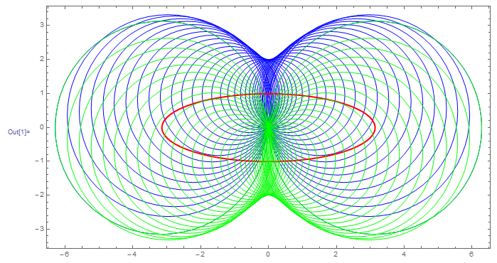
First look at it in 2D

With[{a = Pi, b = 1},
 Graphics[{
    {Blue, Table[Circle[{x, b/a Sqrt[a^2 - x^2]}, b Sqrt[1 + x^2/b^2 - x^2/a^2]], {x, -a, a, a/17}]}, 
    {Red, Thick,Circle[{0, 0}, {a, b}]}, 
    {Green, Table[Circle[{x, -b/a Sqrt[a^2 - x^2]}, b Sqrt[1 + x^2/b^2 - x^2/a^2]], {x, -a, a, a/17}]}}, 
  Frame -> True]
 ]

then produce the solid of revolution. Because analytical calculations can become cumbersome often an visual equivalent procedure is the following: get the contour in 2D of the points depicted and use an interpolating function on it to get the input necessary to run RevolutionPlot3D. To do so one switches from Circle to Disk

R = With[{a = 2 \[Pi], b = 1},
   BooleanRegion[Or, 
    Join[Table[Disk[{x, b/a Sqrt[a^2 - x^2]}, b Sqrt[1 + x^2/b^2 - x^2/a^2]], {x, -a, a, a/17}], 
           Table[Disk[{x, -b/a Sqrt[a^2 - x^2]}, b Sqrt[1 + x^2/b^2 - x^2/a^2]], {x, -a, a, a/17}]
    ]
  ]
];

and discretizes it:

DiscretizeRegion[R]
BoundaryDiscretizeRegion[R]

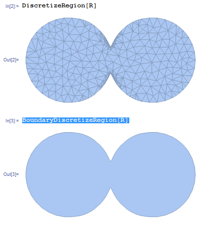
the boundary discretized region is a good candidate to work with in RevolutionPlo3D.