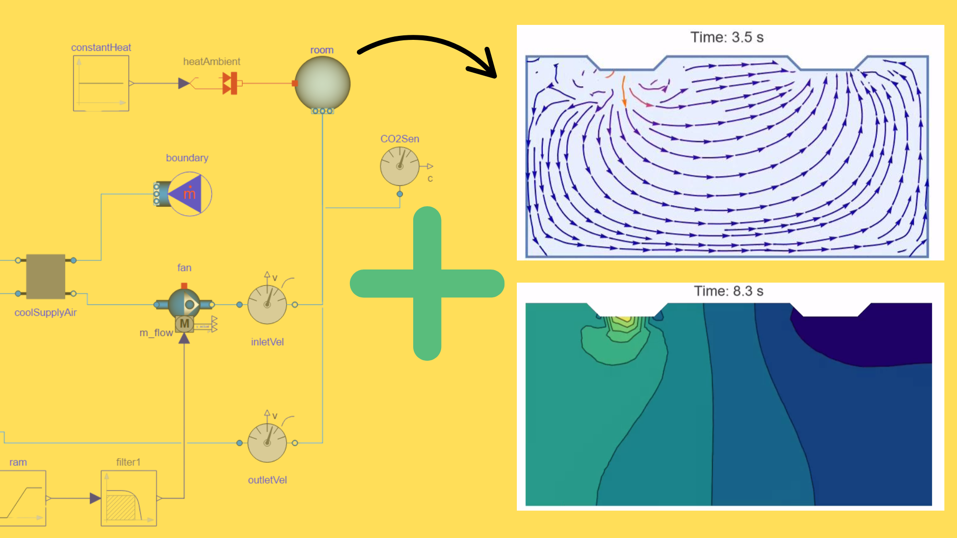
Engineering teams face the same dilemma over and over:

• Oversimplify too much -> you miss airflow dead zones and end up with poor comfort.
• Overcomplicate too soon -> you burn weeks of compute on cases that don't matter

The real answer? A hybrid workflow: start with system models, add detail only when it matters and keep everything connected.

Case Study: Cooling a Room with HVAC

We set out to answer a simple question:

How should an HVAC system be configured to keep a room comfortable while minimizing energy use?

At the system level, Modelica (using the IBPSA library) makes it easy to capture control strategy and system behavior.

Load the model and IBPSA library:

CloudImport[CloudObject["https://www.wolframcloud.com/obj/b9ea8653-2418-4297-a5e8-1f7bcefb18d6"]];

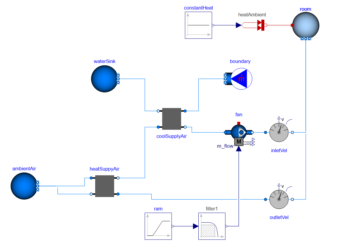
Check the model diagram:

model = SystemModel["RoomHeating"];
model[{"Diagram", Frame -> False}]

Plot the simulation results:

sim = SystemModelSimulate[model, 120];
SystemModelPlot[sim, PlotRange -> All, TargetUnits -> {"Seconds", Automatic}]

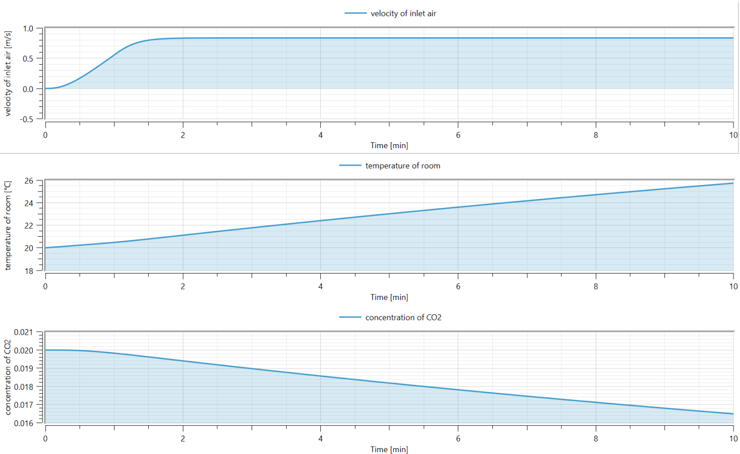
• Inlet velocity ramps up from near zero to about 0.8 m/s in the first two minutes.
• The room temperature shows how quickly the heating takes effect.
• CO2 concentration trends reveal long-term air quality impacts.

These quick insights already help test strategies without heavy computation. But they don't tell us why one corner of the room feels stale or how inlet and outlet duct placement affects airflow.

Adding Detail with FEM

This is where finite element modeling (FEM) adds value.

By extending the workflow, we can see:

• Velocity fields -- stream plots reveal how air jets circulate, pinpointing dead zones with poor mixing.
• Pressure distribution -- contour plots expose back pressure at outlets, highlighting inefficiencies in fan energy use.

For this demonstration, I combined System Modeler (Modelica) for system behavior with the Wolfram Language FEM framework for spatial detail.

Load the Finite Element package:

Needs["NDSolve`FEM`"]

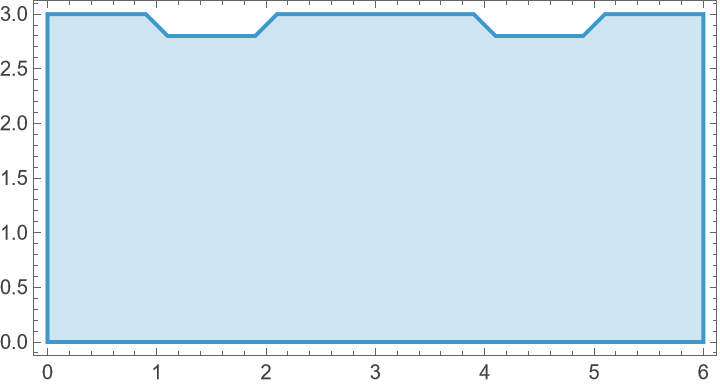
Set up and visualize the geometry:

region = Polygon[{{0, 0}, {6, 0}, {6, 3}, {5.1, 3}, {4.9, 2.8}, {4.1, 2.8}, {3.9, 3}, {2.1, 3}, {1.9, 2.8}, 1.1, 2.8}, {0.9, 3}, {0,3}}];
RegionPlot[region, AspectRatio -> Automatic]

Define properties of the material:

tpars = <|"ReynoldsNumber" -> 1000, "Material" -> Entity["Chemical", "Air"]|>;

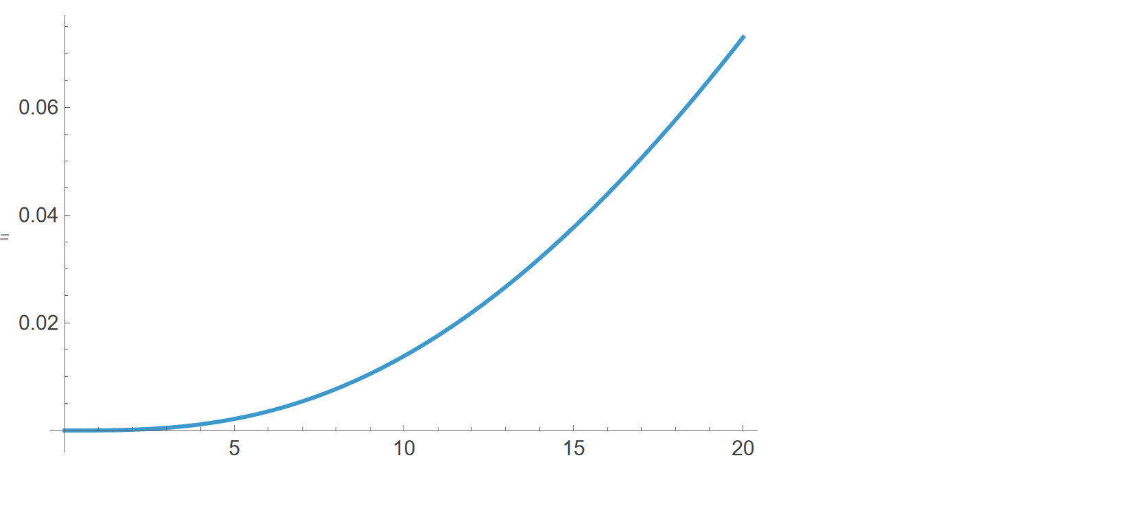
Create inlet velocity data:

data = Interpolation[{#, sim["inletVel.v"][#]} & /@ Range[0, 120, 1], InterpolationOrder -> 2];
Plot[data[t], {t, 0, 20}]

Set up boundary conditions:

bcs = {
   DirichletCondition[{u[t, x, y] == 0, v[t, x, y] == -data[t]}, 1.1 < x < 1.9 && y == 2.8],
   DirichletCondition[{u[t, x, y] == 0, v[t, x, y] == 0}, 0 <= x <= 6  && y < 2.8],
   DirichletCondition[{u[t, x, y] == 0, v[t, x, y] == 0}, 0 <= x <= 6  && y > 2.8],
   DirichletCondition[p[t, x, y] == 0, 4.1 < x < 4.9 && y == 2.8]
   };

Set up initial conditions:

ic = {u[0, x, y] == 0, v[0, x, y] == 0, p[0, x, y] == 0}

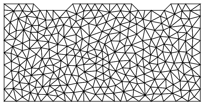
Create a mesh:

mesh = ToElementMesh[region, MaxCellMeasure -> 0.01];
mesh["Wireframe"]

Set up model variables:

tvars = {{u[t, x, y], v[t, x, y], p[t, x, y]}, t, {x, y}};

Define a flow PDE model:

op = FluidFlowPDEComponent[tvars, tpars];

Solve the PDE:

tEnd = 20;
AbsoluteTiming[
 Monitor[{uVel, vVel, pressure} = 
    NDSolveValue[{op == {0, 0, 0}, bcs, ic}, {u, v, p}, 
     Element[{x, y}, mesh], {t, 0, tEnd}, 
     Method -> {"PDEDiscretization" -> {"MethodOfLines", 
         "SpatialDiscretization" -> {"FiniteElement", 
           "InterpolationOrder" -> {u -> 2, v -> 2, p -> 1}}}},
     EvaluationMonitor :> (monitor = Row[{"t = ", CForm[t]}])];, 
  monitor]]

Get the velocity distribution inside the room:

frames = StreamPlot[
    {uVel[#, x, y], vVel[#, x, y]},
    {x, y} \[Element] region,
    PlotLabel -> "Time: " <> ToString[#] <> " s",
    Frame -> False,
    AspectRatio -> Automatic] & /@ Range[0, tEnd, 5];

Create a video from the frames:

FrameListVideo[frames]

Get the pressure distribution inside the room:

framesPressure = ContourPlot[
    pressure[#, x, y],
    {x, y} \[Element] region,
    ColorFunction -> "BlueGreenYellow",
    PlotLabel -> "Time: " <> ToString[#] <> " s",
    Frame -> False, AspectRatio -> Automatic] & /@ Range[0, tEnd, 5]

Create a video from the pressure distribution frames:

FrameListVideo[framesPressure]

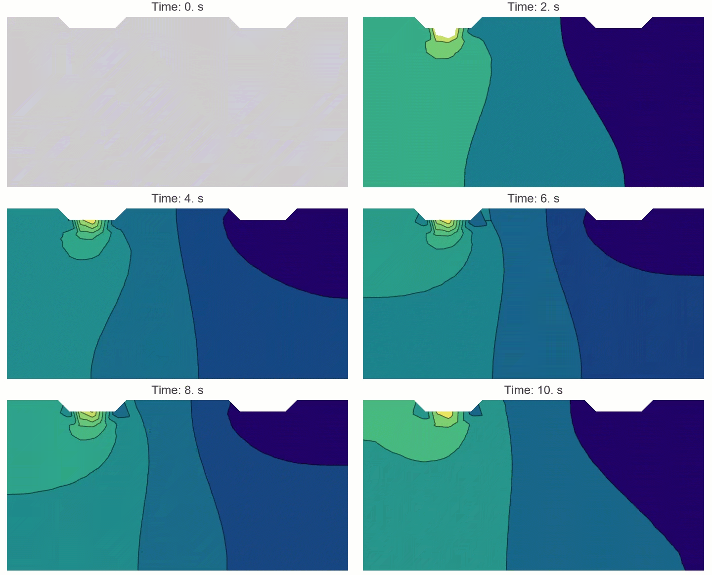
Instead of a single airflow number, we now see exactly how air moves, corner by corner, second by second.

Why This Matters

This integrated workflow eliminates two big pain points:

• System-only models -> fast, but blind to spatial effects.
• FEM-only models -> accurate, but too slow for design iteration.

With System Models + FEM:

• System Models handles system intelligence (controls, operating scenarios).
• FEM provides spatial insight when and where it's needed.
• Together, they build a digital twin that's accurate and efficient.

As engineers, our job isn't to simulate everything---it's to simulate what matters.

The future lies in modular, hybrid modeling pipelines like this one, where Modelica provides system context and FEM provides spatial detail.