In this post, I’ll walk you through some of the new possibilities in System Modeler version 14.3.

Engineering in today’s world

As we enter the age of renewables and smart, connected systems, some challenges emerge across industries.

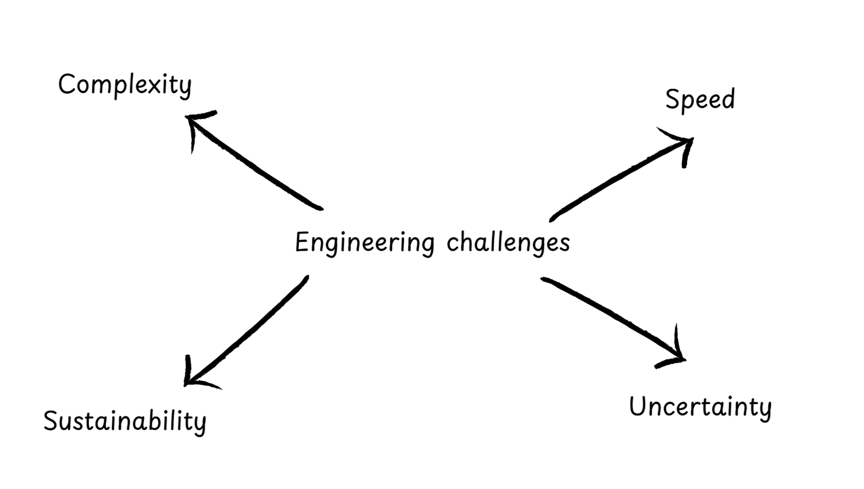
• Complexity: Systems aren’t standalone anymore—an electric vehicle is also a powertrain, a battery, a thermal system, and a software stack, all tightly coupled.
• Sustainability: Every design decision now has to balance performance with energy efficiency, emissions, and long-term environmental impact.
• Speed: The pressure to deliver faster means we need tools that shorten prototyping cycles and reduce manual work.
• Uncertainty: Real-world conditions—like weather, usage patterns, or supply variability—are unpredictable, but designs still need to perform reliably.

These four challenges—complexity, sustainability, speed, and uncertainty—are what define modern engineering.

And the question is:

How do we design systems that don’t fail under these pressures?

What If...

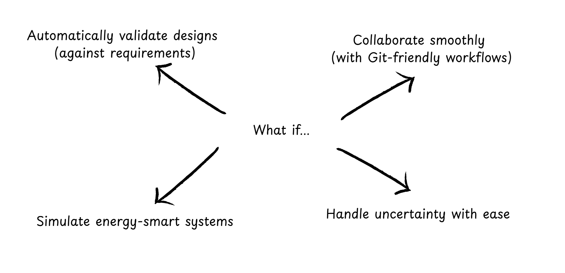
Let’s flip that challenge around.

What if we could design in a way that anticipates these uncertainties?

What if we could:

• Validate thousands of scenarios automatically,
• Build models of microgrids or HVAC systems quickly with ready-made components,
• Iterate on designs faster, with LIVE tuning,
• And collaborate seamlessly across teams.

That’s the vision driving System Modeler 14.3. Let’s see how it comes to life in the new capabilities and libraries we’ve added.

Challenge 1: Safe & Reliable Design under Uncertainty

Let’s start with the first challenge: designing for reliability under uncertainty.

Testing a single scenario is easy. But in reality, a design must perform across all conditions—different drive cycles, weather, and vehicle loads.

Here’s an EV thermal management model. Imagine you’re the thermal engineer responsible for keeping the battery within safe limits.

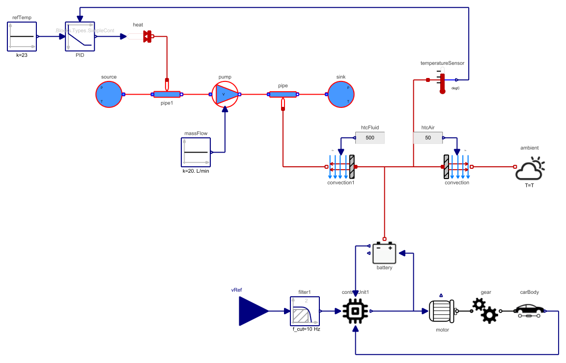
Here, you can see the battery connected to its cooling system. We’ll link this to a drive cycle and simulate the thermal performance.

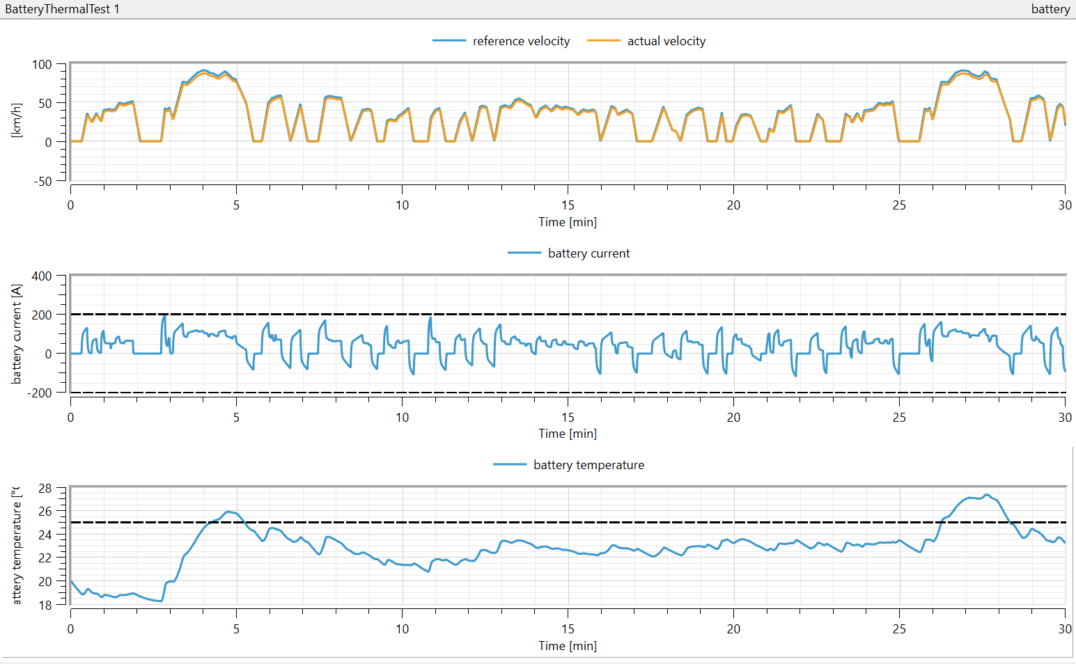
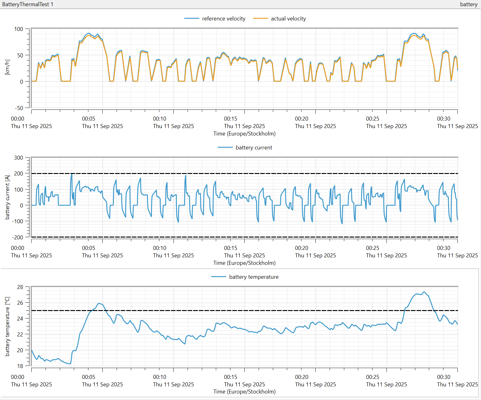
The plots show three things: the velocity profile of the car, the battery current, and the battery temperature.

Now, there are clear requirements:

• Battery current must stay below 200 A,
• Battery temperature must not remain above 25 °C for more than 4 minutes.

In this first simulation, the results look okay. Current is within limits, and although the temperature goes above 25 °C, it doesn’t stay there long enough to break the requirement.

But—this is just one scenario.

What about real-world conditions? Stop-and-go traffic, hot summer days, or carrying heavy loads? Running all these cases manually is tedious—and analyzing whether each one passes requirements usually takes a lot of scripting.

Automatically Test Requirements across Any Number of Scenarios

With version 14.3, we introduced a requirement specification language with functions like SystemModelValidate. These let you validate designs directly against performance and safety requirements.

Using these functions, you can check behavior over time, manage uncertainty, and detect edge-case failures early in the design process.

Here’s how it works in our EV example:

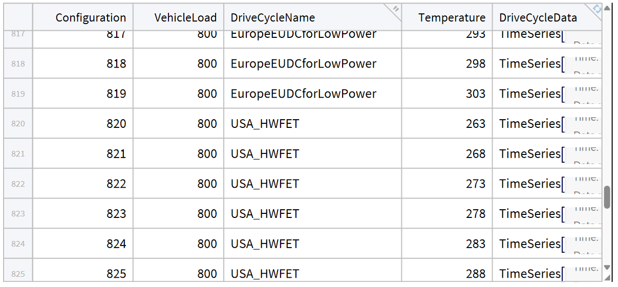
• You could always run thousands of simulations in parallel using SystemModelSimulate, each with different drive cycles, loads, and ambient conditions.

   sims = Quiet@SystemModelSimulate[
          "ThermalManagement.BatteryThermal",
          <|
           "Inputs" -> {"vRef" -> refVelocities},
           "ParameterValues" -> {"T" -> temperatures, "load" -> vehicleLoads}
           |>
          ]; 
  

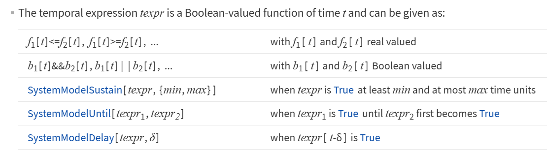
• Now, with version 14.3, we can express requirements directly. Using functions like SystemModelAlways, we encode conditions such as:

• Battery temperature must not exceed 25 °C for more than 5 minutes,

• Start evaluating only after 300 seconds, to skip startup effects.

  req = SystemModelAlways[t, 
         300 <= t, ! 
          SystemModelSustain[
           "temperatureSensor.T"[t] > 25, {Quantity[4, "Minutes"], Infinity}]];
  

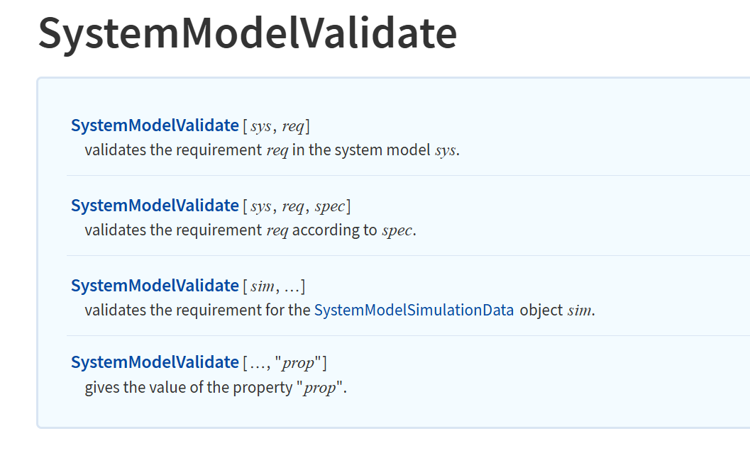
• We then pass this requirement to SystemModelValidate. The function checks the simulations and reports the results.

  validationResult = SystemModelValidate[sims, req]
  

• In this case, one test failed.

• The system also records where, when, and under which configurations failures occur, so you can trace them.

  validationResult["FailurePlot"]
  

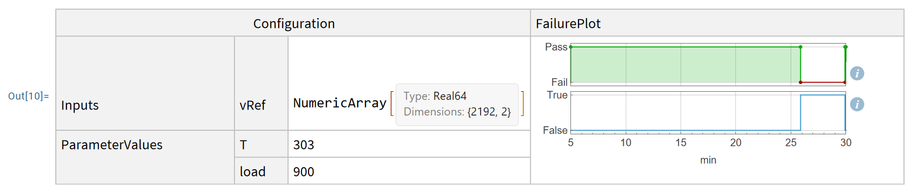
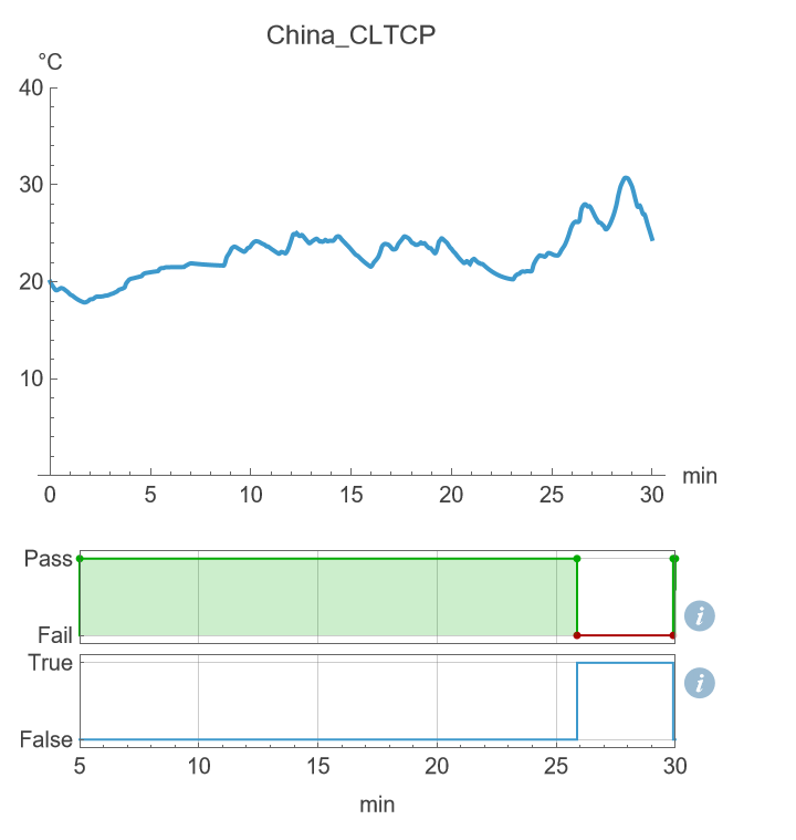
• Here, the failure is in the China drive cycle. The failure plot shows the battery temperature staying above 25 °C for over 4 minutes.

In practice, this replaces hours of manual validation with a single function call—delivering insights much earlier in the workflow.

So here’s a summary of what that means in practice. I can simply:

• Run the EV drive cycle model,
• Provide a list of drive cycles and operating conditions,
• State my requirements—like current or temperature limits,
• And tell the function to report all violations.

That’s it: one function call.

Suddenly, I’ve validated my design across thousands of scenarios, without writing custom scripts for each case.

And here’s the big shift: engineers can now spend their time making design decisions, not building validation code.

This saves enormous amounts of time—what used to take hours now takes minutes.

More importantly, it transforms the workflow:

• You can validate much earlier in the design phase,
• You can test far more scenarios than before,
• And you can build safer, more reliable systems, because problems are caught automatically.

That’s how System Modeler 14.3 addresses the first challenge: safe, reliable design under uncertainty.

Next, let’s move on to the second challenge: energy systems and the climate transition.

Challenge 2: Climate & Energy Transition

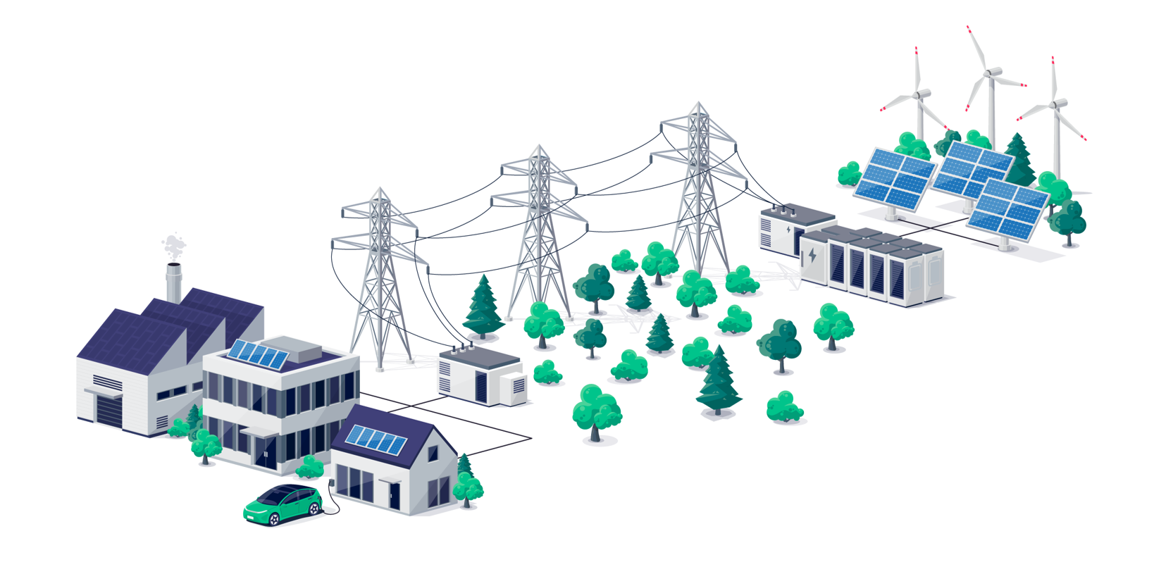
Energy systems today must integrate renewables, grids, and buildings with rooftop solar—and they have to do so reliably.

The problem is that building these models from scratch is often slow and complex.

That’s why System Modeler 14.3 introduces support for energy libraries:

• The Photovoltaics Library for PV and grid integration,
• The Power Grids and Power Systems Libraries for transient grid modeling,
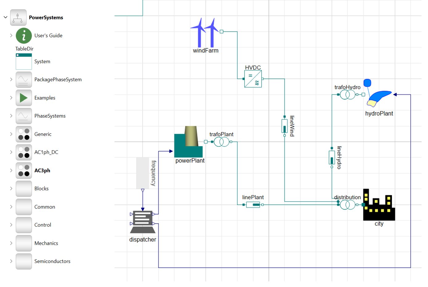
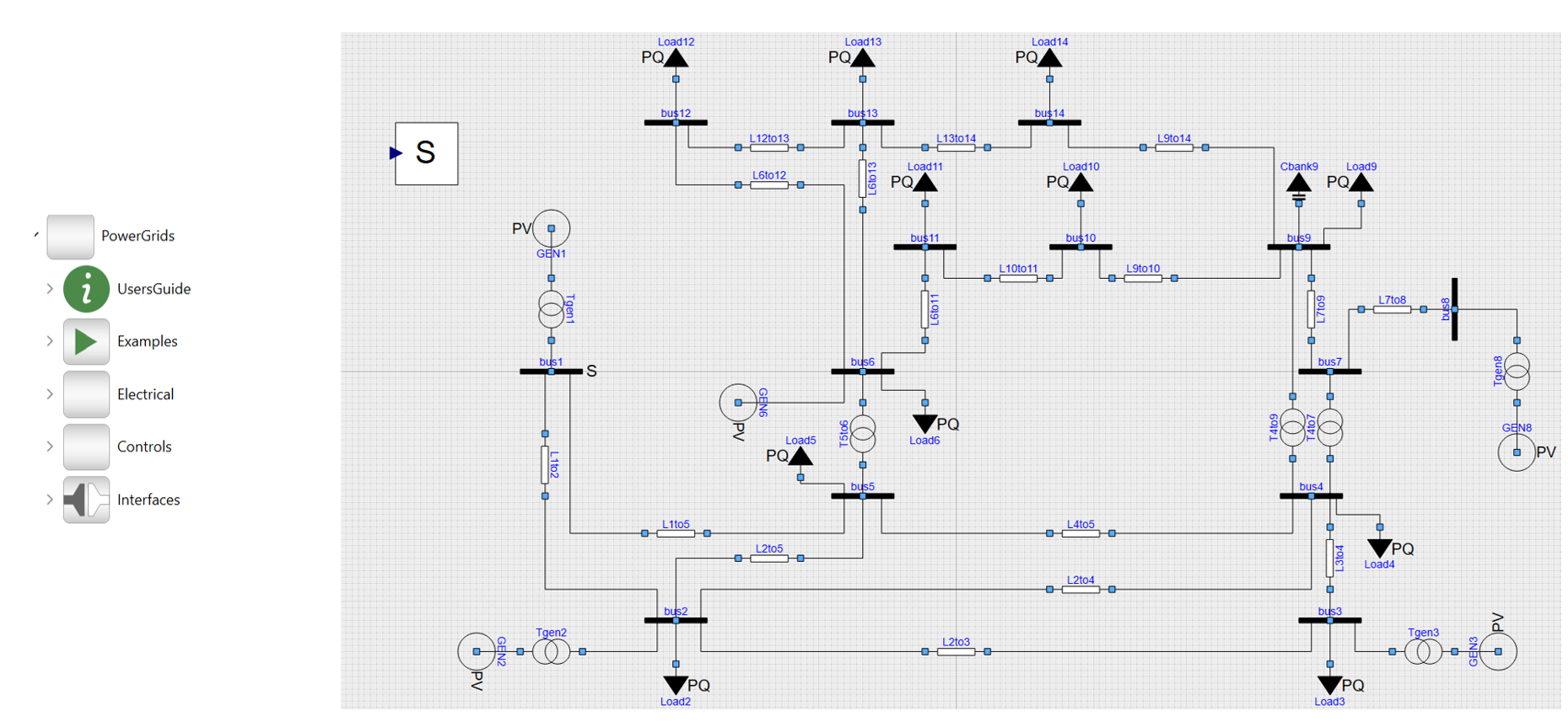
• And the IBPSA Buildings Library for designing HVAC systems.

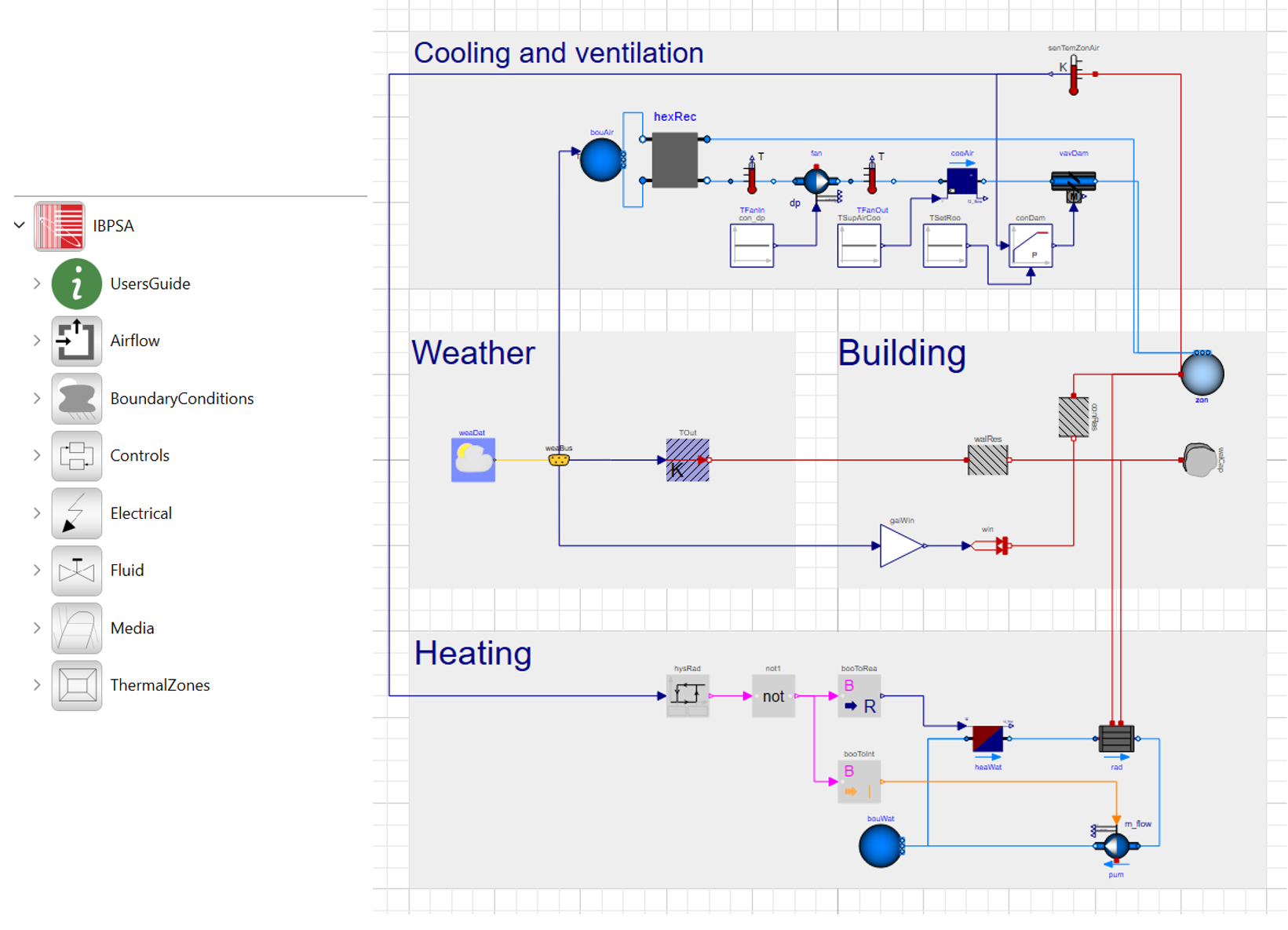
Together, these libraries let you model not just one component, but the entire ecosystem—from rooftop solar all the way down to heat exchangers, pipes and valves to model HVAC systems.

Maintain Thermal Comfort inside a Room

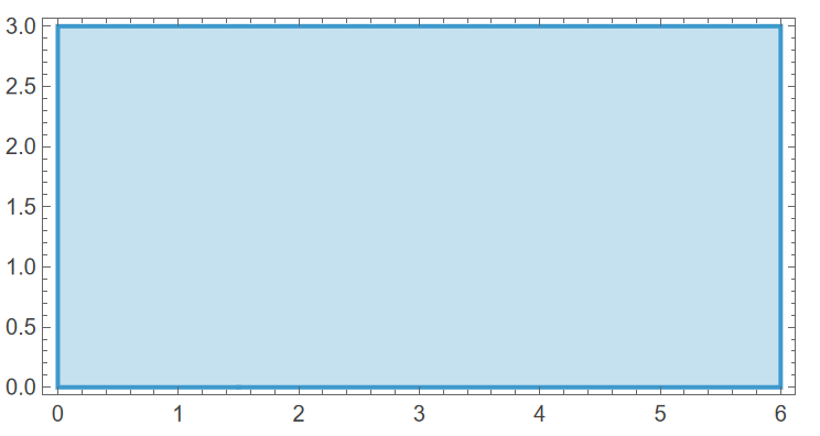
Let’s look at an example. Let’s say you are a HVAC engineer who is tasked with maintaining thermal comfort in a room of height 3m and width 6m.

Your job is to:

• Keep indoor conditions comfortable,
• Ensure good air quality,
• And minimize energy consumption in a building.

There are 2 things you have to design:

How should the HVAC system, including the flow rates, pump sizes and heat exchangers, be designed?

How should the inlet and outlet ducts be placed to ensure even airflow inside the room?

Let’s answer the first question:

With the IBPSA library, you have access to components such as fans, pumps, ducts, and heat exchangers that you can readily use and build a full system model.

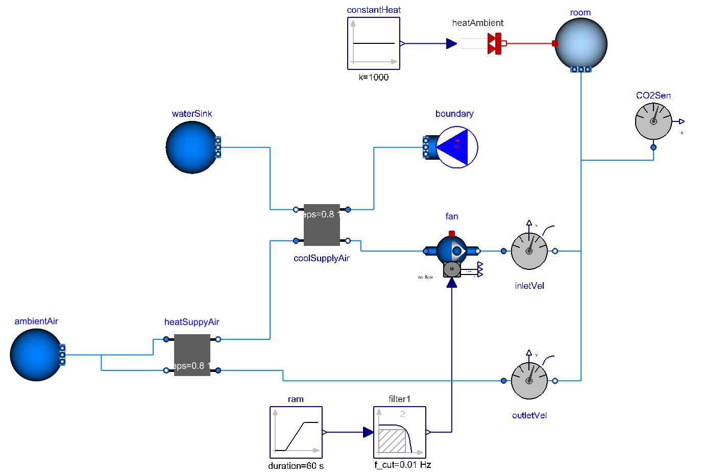
In this case, air from the ambient is heated through a heat exchanger, then cooled using another heat exchanger. Then, they were sent to the room.

In heat exchanger 1, the outlet air from the room is used to heat the inlet air, whereas in heat exchanger 2, water is used to cool the air.

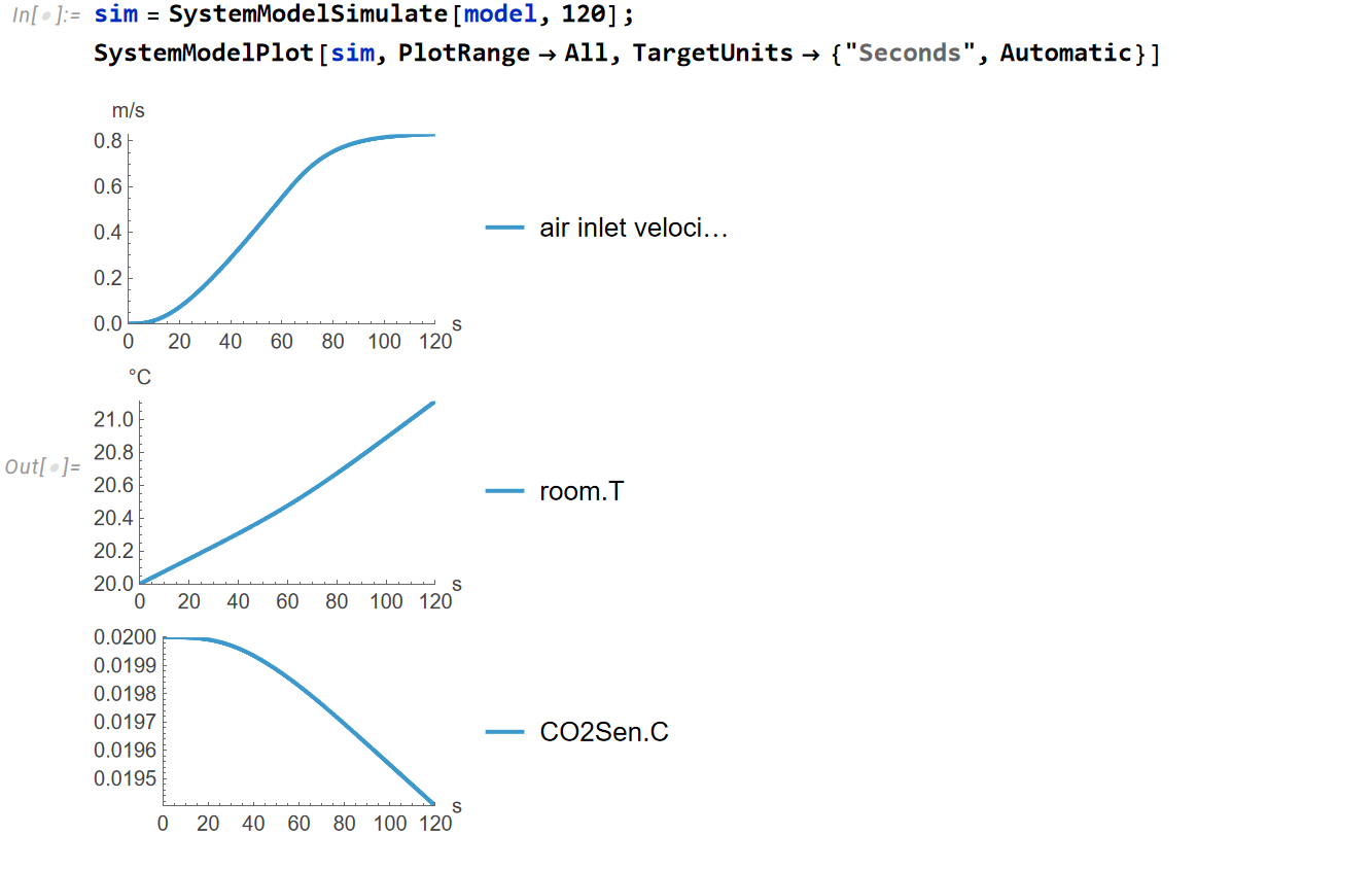
And once the model is built, you can immediately start simulating how the building behaves under different conditions. You can control the air inlet velocity, water mass flow rate, and track the room temperature along with the CO2 levels in the room to maintain comfort.

Now let’s answer the second question—duct placement.

We can use the system model for boundary conditions, and then apply FEM in Wolfram Language to simulate airflow and pressure inside the room.

Scenario 1 – ducts pointing downward:

• Velocity plots show strong jets hitting the floor, creating uneven circulation.
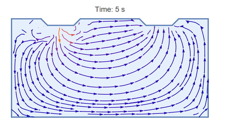
• Pressure is high near inlets but drops off in the back.

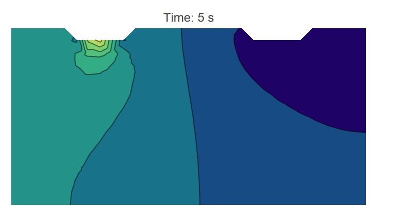
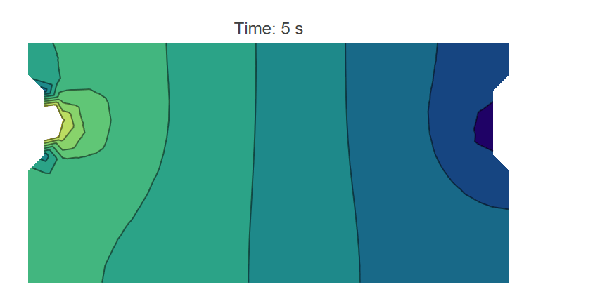
Scenario 2 – ducts pointing sideways:

• Velocity distribution is smoother, mixing is more even.
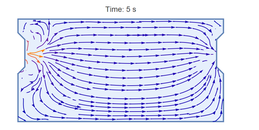
• Pressure is balanced across the room.

Now, as the HVAC designer, you can clearly weigh the trade-offs:

• Downward ducts are cheaper to install but less effective.
• Sideways ducts improve comfort but require more ductwork and cost.

With System Modeler + FEM, you’re able to compare these design options directly.

For an HVAC designer, this workflow changes everything:

• You can model the entire system—from pipes and heat exchangers to airflow in a single room.
• You can compare multiple designs quickly and make informed trade-offs.
• And you can communicate results visually, making it easier to align with architects, managers, and clients.

That’s the second challenge: tackling the climate and energy transition by making energy systems easier to design, test, and optimize.

Challenge 3: Faster Iteration & Insight

Our third challenge is iteration speed.

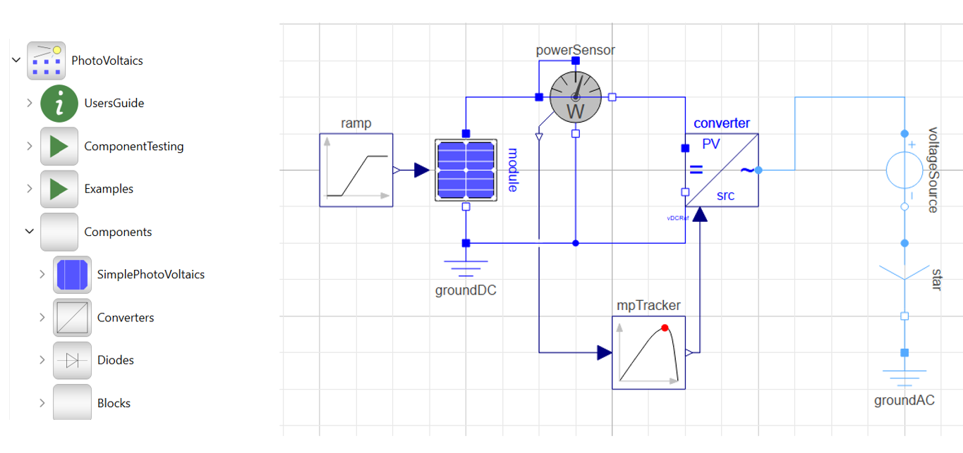
Imagine you’re a solar design engineer tasked with configuring a rooftop PV system.

You need to decide:

• How many modules to connect in series,
• How many to connect in parallel,
• And how the system performs under different configurations.

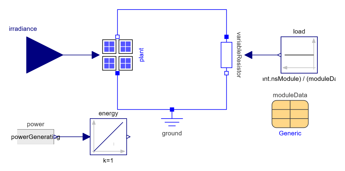
Here you see a solar plant connected to a fixed load. If we simulate this model, we can examine how power, voltage, and current change as we vary the number of modules.

Traditionally, exploring different configurations meant stopping and restarting the simulation for each parameter set.

With version 14.3, we can do this differently. We can:

• Run a simulation once in real-time,
• Adjust parameters—like number of series modules or parallel modules—in real time,
• And instantly see the impact on power output and electrical characteristics.

We can even track parameter history and compare multiple configurations, all in a single run.

For our rooftop solar engineer, this means less time waiting, more time designing and optimizing.

Calendar-time simulation

There’s another new feature in 14.3 that makes results much more intuitive: calendar-time simulation.

In earlier versions, results were always shown in generic simulation time—seconds, minutes, or related time units. That makes it hard to connect to real-world performance.

With version 14.3, you can now enable the “Use date and time” option in settings. This lets you anchor your simulation to a specific calendar date.

The same applies in the Wolfram Language. When plotting results, you can set an epoch—for example, start on January 1st, 2015—and even bring in real solar irradiance data from databases like PVGIS. Then run the PV model across an entire year.

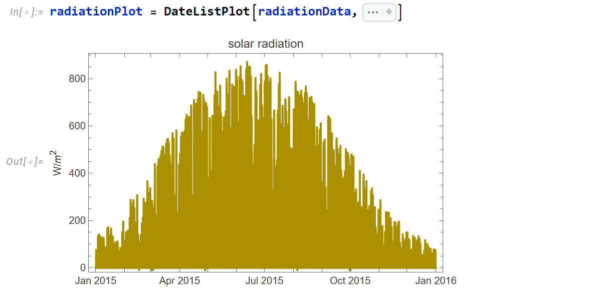
SystemModelPlot[
 "PVModule.PVModulePower1",
 {"plant.powerGenerating"},
 Quantity[1, "Years"],
 <|
  "Inputs" -> {"irradiance" -> TimeSeriesShift[radiationData, {{0}}]}
  |>,
 PlotRange -> All,
 Method -> {"Epoch" -> DateObject[{2015, 1, 1}, "Day"]}
 ]

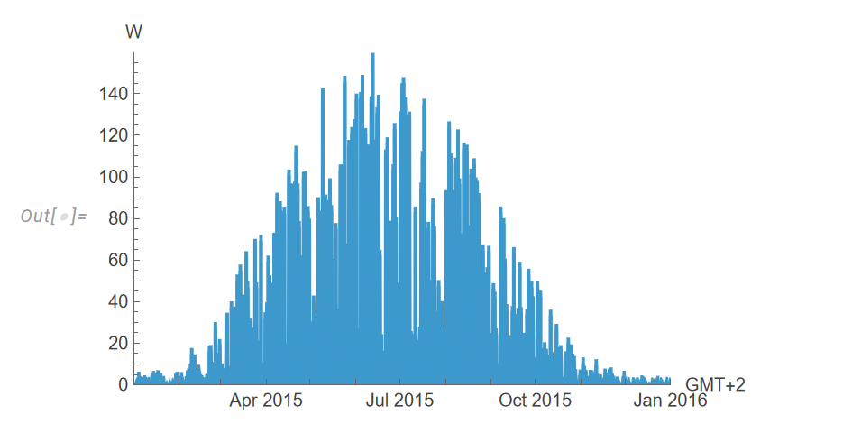The outputs are plotted directly on a calendar scale—so you can immediately compare performance in winter versus summer.

This makes it far easier for both engineers and stakeholders to connect simulation results to real-world experience.

So what does this mean for our solar design engineer?

• They can configure rooftop systems in real time without endless restart cycles,
• Track the history of their design adjustments as they go,
• And evaluate system performance across an actual calendar year.

This accelerates prototyping cycles, makes iteration more intuitive, and leads to better designs in less time.

So that’s the third challenge: faster iteration and deeper insight through live tuning and calendar-time simulation.

And More...

Beyond the three challenges, System Modeler 14.3 also includes some smaller but very practical improvements.

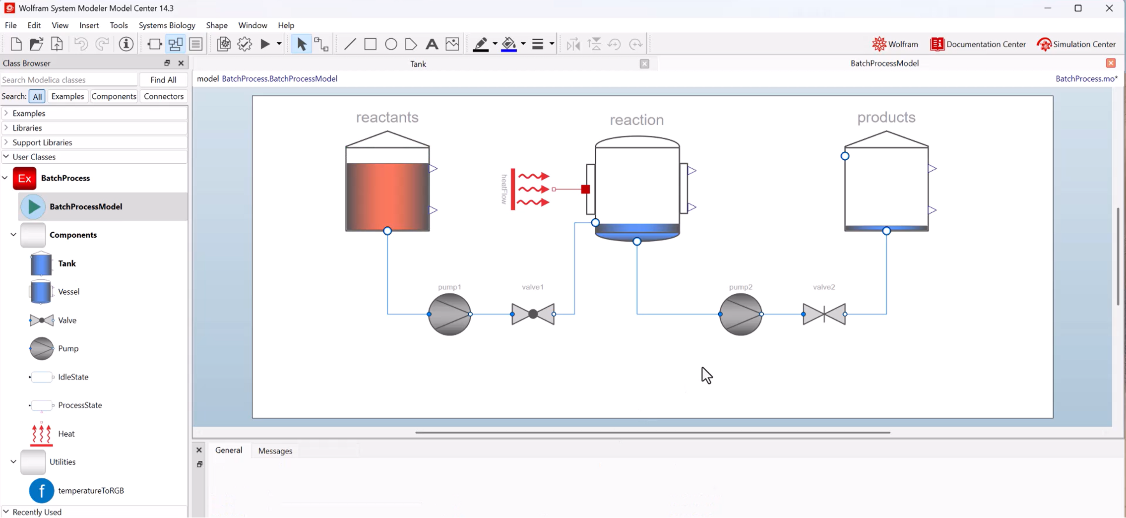
One improvement is that you can modify an icon based on the parameter values. For example, in this process plant model, the color of the tank depends on the temperature of the fluid. That means you can see configurations at a glance, and spot errors directly in the diagram—without digging into code.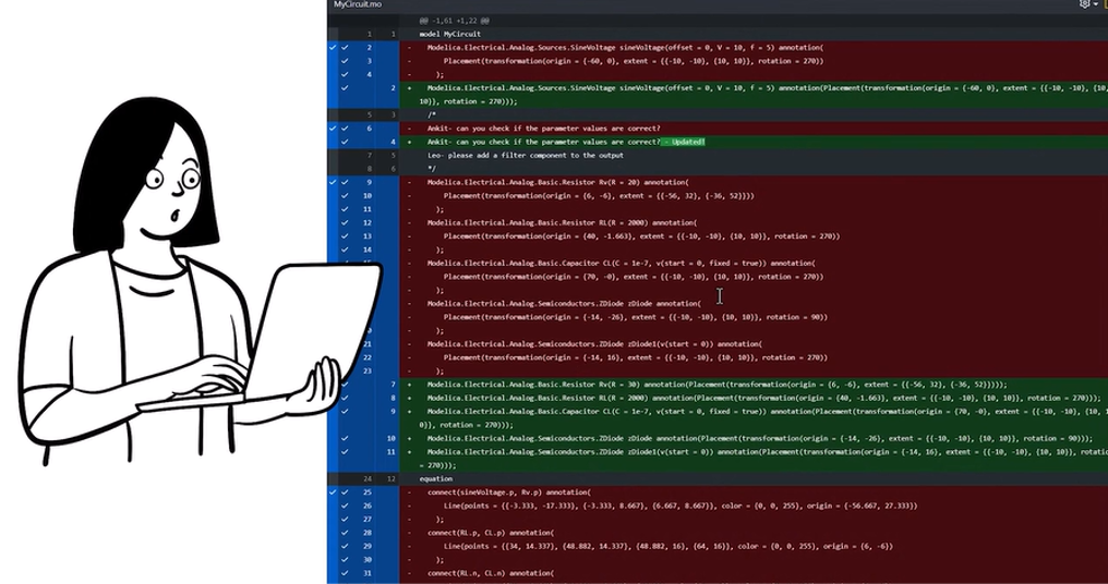

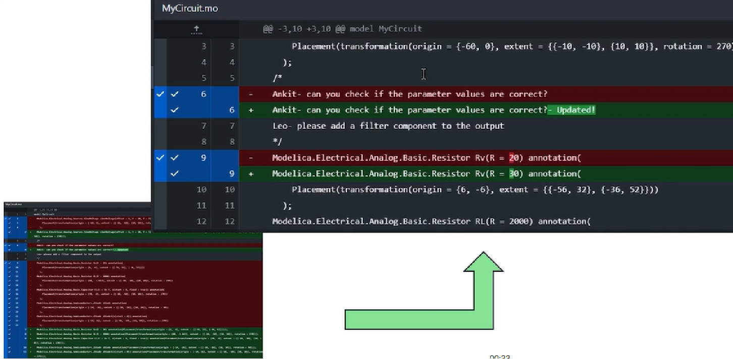
Another big help for collaboration: the underlying Modelica code is now Git-friendly. Formatting is cleaner, diffs are easier to read, and version control flows more smoothly. For larger projects, this saves a lot of time in reviewing and merging changes.

These might sound like small details, but they make a big difference:

• Catch configuration issues earlier, before they become costly,
• Collaborate more smoothly with colleagues, thanks to cleaner version control.

Summary

With System Modeler 14.3, we’ve seen how you can:

• Build safer designs under uncertainty by validating thousands of scenarios,
• Model climate and energy systems more easily, from rooftop solar to airflow in a single room,
• And iterate faster with live tuning and calendar-time simulation.
• On top of that, you also get practical improvements for visualization and collaboration—like configuration-aware icons and Git-friendly formatting.

If you’d like to explore more:

• The What’s New page gives a deeper dive into the new features,
• And the System Modeler overview page is a great place to start if you’re new to the tool.

I invite you to explore these capabilities and see how they can fit into your own projects.