An infographic for the MRB constant records:
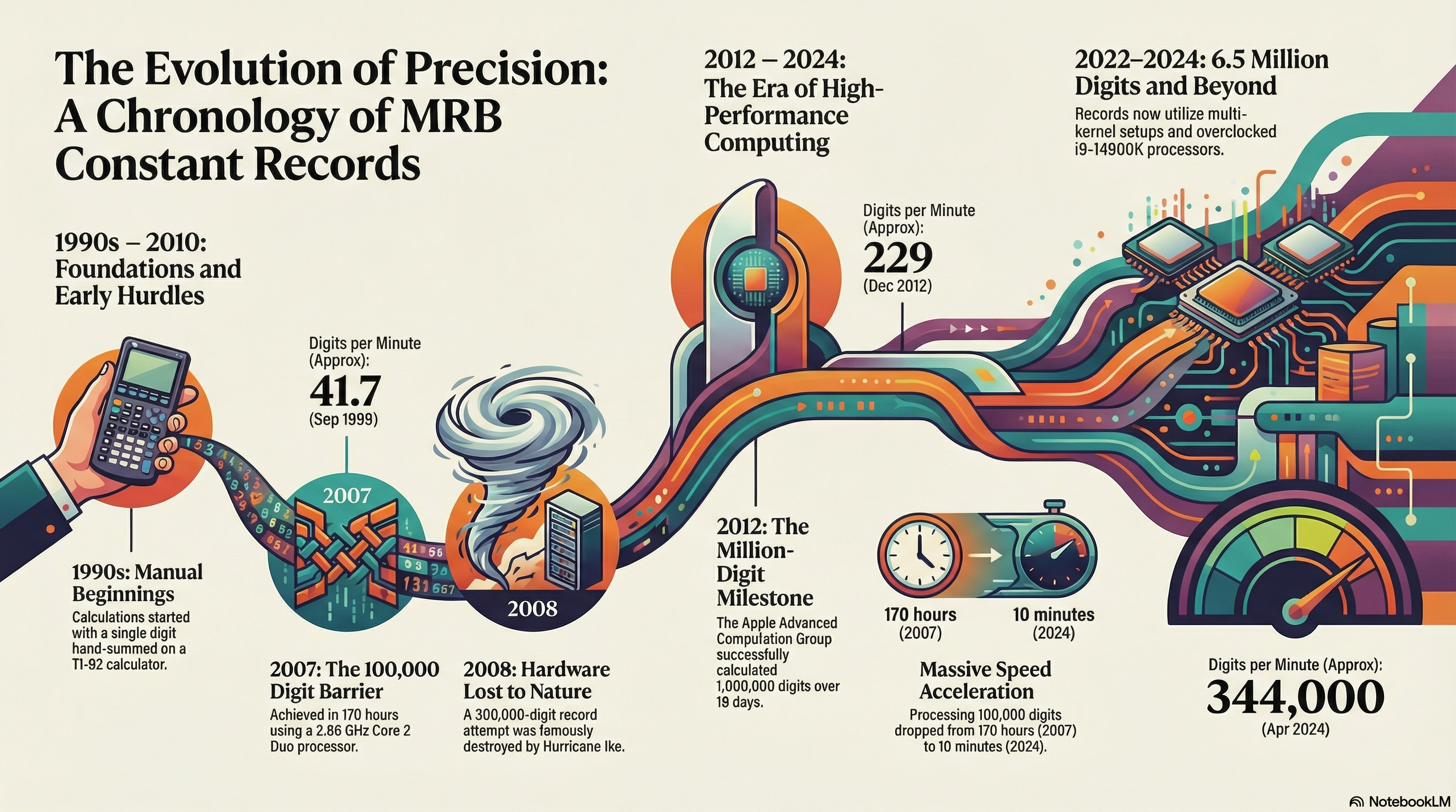
MRB Constant Records,
Google Open AI Chat CPT gave the following introduction to the MRB constant records:
It is not uncommon for researchers and mathematicians to compute large
numbers of digits for mathematical constants or other mathematical
quantities for various reasons. One reason might be to test and
improve numerical algorithms for computing the value of the constant.
Another reason might be to use the constant as a benchmark to test the
performance of a computer or to compare the performance of different
computers. Some people may also be interested in the mathematical
properties of the constant, and computing a large number of digits can
help to reveal patterns or other features of the constant that may not
be apparent with fewer digits. Additionally, some people may simply
find the process of calculating a large number of digits to be a
challenging and rewarding intellectual pursuit.
My inspiration to compute a lot of digits of CMRB came from this archived linked website by Simon Plouffe.
There, computer mathematicians calculate millions, then billions of digits of constants like pi, when with only 65 decimal places of pi, we could determine the size of the observable universe to within a Planck length (where the uncertainty of our measure of the universe would be greater than the universe itself)!
In contrast, 65 digits of the MRB constant "measures" the value of -1+ssqrt(2)-3^(1/3) up to n^(1/n) where n is 1,000,000,000,000,000,000,000,000,000,000,000,000,000,000,000,000,000,000,000,000,000,000, which can be called 1 unvigintillion or just 10^66.
And why compute 65 digits of the MRB constant? Because having that much precision is the only way to solve such a problem as
1465528573348167959709563453947173222018952610559967812891154^ m-m,
where m is the MRB constant, which gives the near integer "to beat
all,"
200799291330.9999999999999999999999999999999999999999999999999999999999999900450...
And why compute millions of digits of it? uhhhhhhhhhh.... "Because it's there!" (...Yeah, thanks George Mallory!)
And why?? (c'est ma raison d'être!!!)
So, below are reproducible results with methods. The utmost care has been taken to assure the accuracy of the record number of digit calculations. These records represent the advancement of consumer-level computers, 21st-century Iterative methods, and clever programming over the past 23 years.
Here are some record computations of CMRB. Let me know if you know of any others!
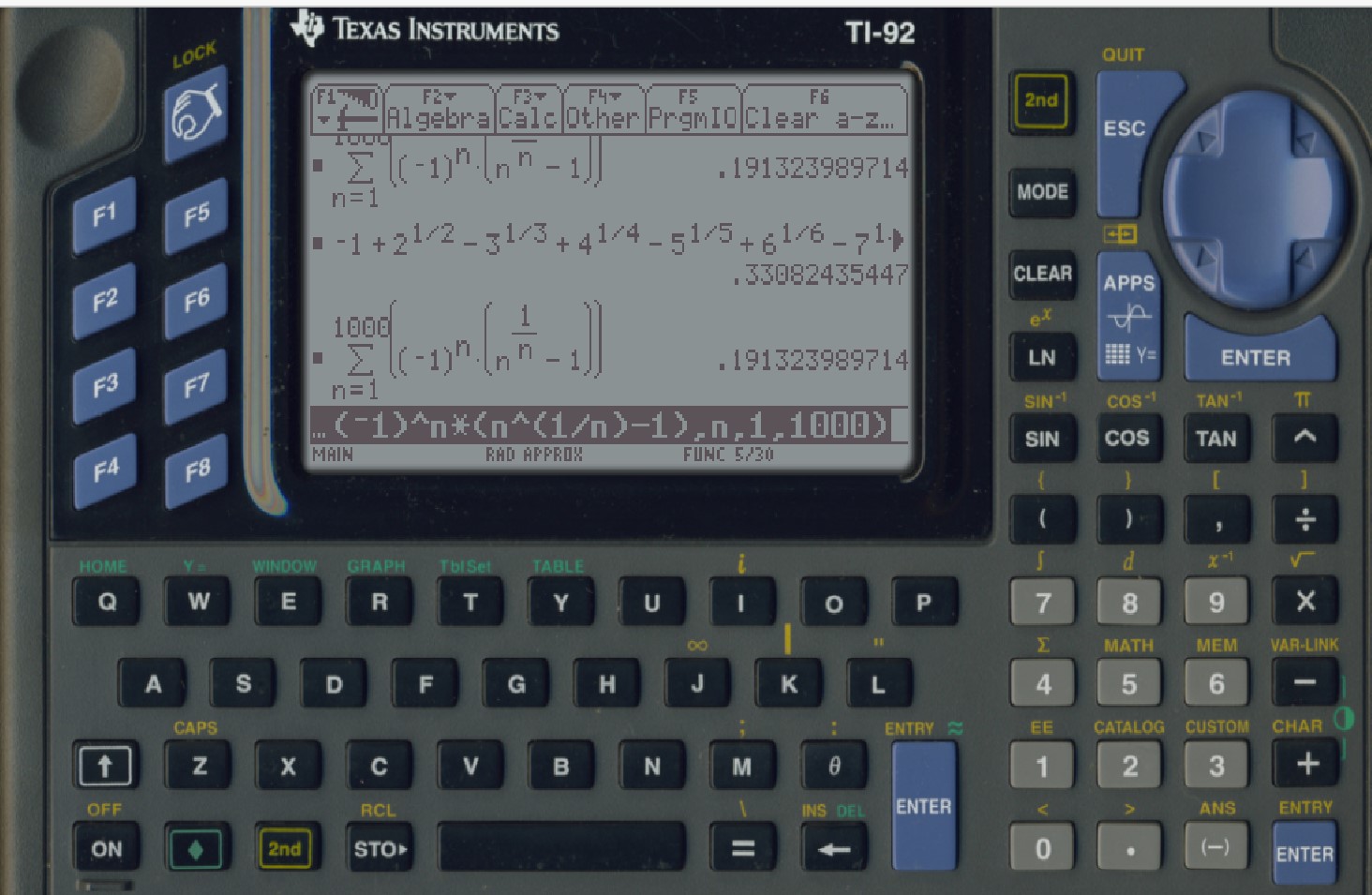
1 digit of the
CMRB with my TI-92s, by adding -1+sqrt(2)-3^(1/3)+4^(1/4)-5^(1/5)+6^(1/6)... as far as practicle, was computed. That first digit, by the way, was just 0. Then by using the sum key, to compute
$\sum _{n=1}^{1000 } (-1)^n \left(n^{1/n}\right),$ the first correct decimal i.e. (.1). It gave (.1_91323989714) which is close to what Mathematica gives for summing to only an upper limit of 1000.
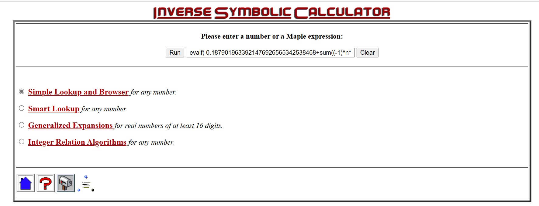
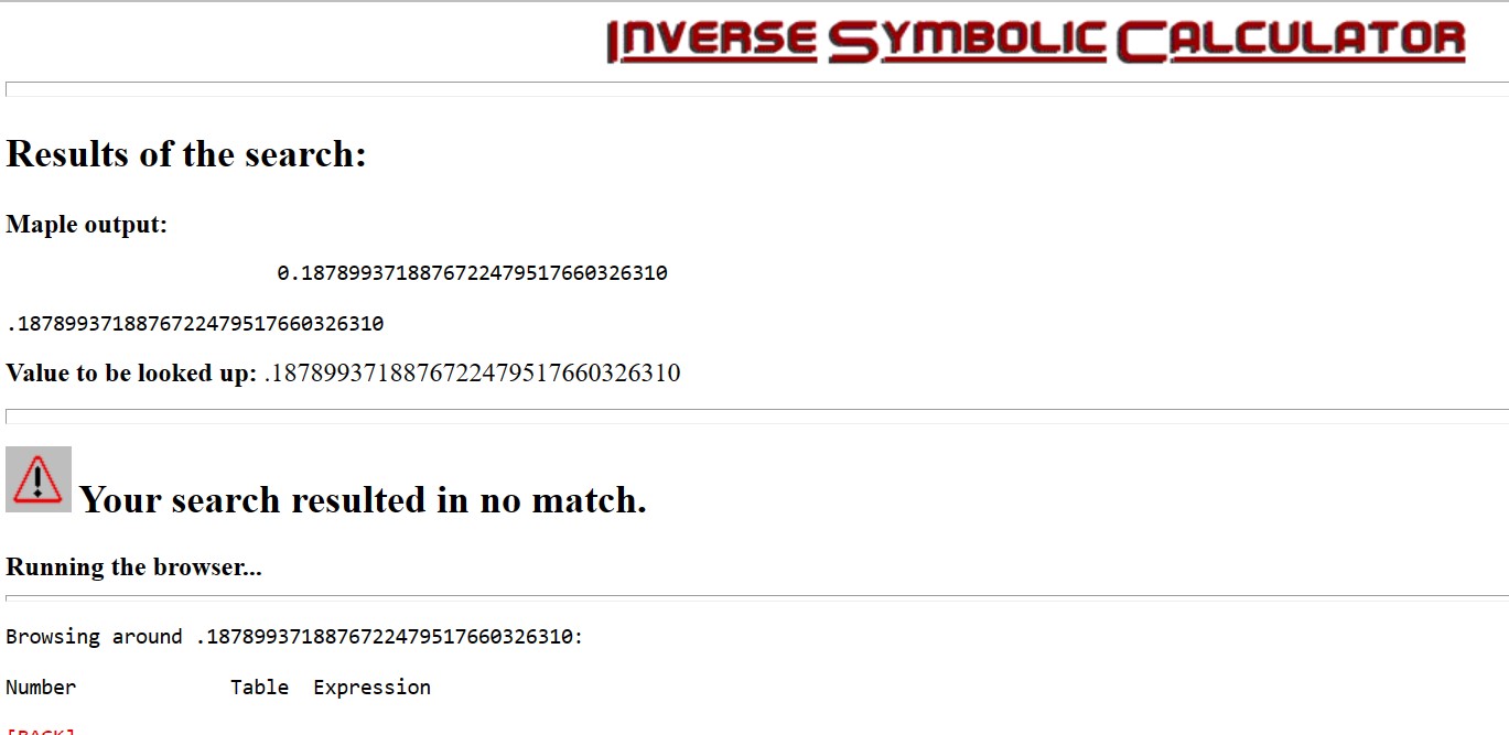
4 decimals(.1878) of CMRB were computed on Jan 11, 1999, with the Inverse Symbolic Calculator, applying the command evalf( 0.1879019633921476926565342538468+sum((-1)^n* (n^(1/n)-1),n=140001..150000)); where 0.1879019633921476926565342538468 was the running total of t=sum((-1)^n* (n^(1/n)-1),n=1..10000), then t= t+the sum from (10001.. 20000), then t=t+the sum from (20001..30000) ... up to t=t+the sum from (130001..140000).
5 correct decimals (rounded to .18786), in Jan of 1999, were drawn from CMRB using Mathcad 3.1 on a 50 MHz 80486 IBM 486 personal computer operating on Windows 95.
9 digits of CMRB shortly afterward using Mathcad 7 professional on the Pentium II mentioned below, by summing (-1)^x x^(1/x) for x=1 to 10,000,000, 20,000,000, and many more, then linearly approximating the sum to a what a few billion terms would have given.
500 digits of CMRB with an online tool called Sigma on Jan 23, 1999. See [http://marvinrayburns.com/Original_MRB_Post.html][6] if you can read the printed and scanned copy there.
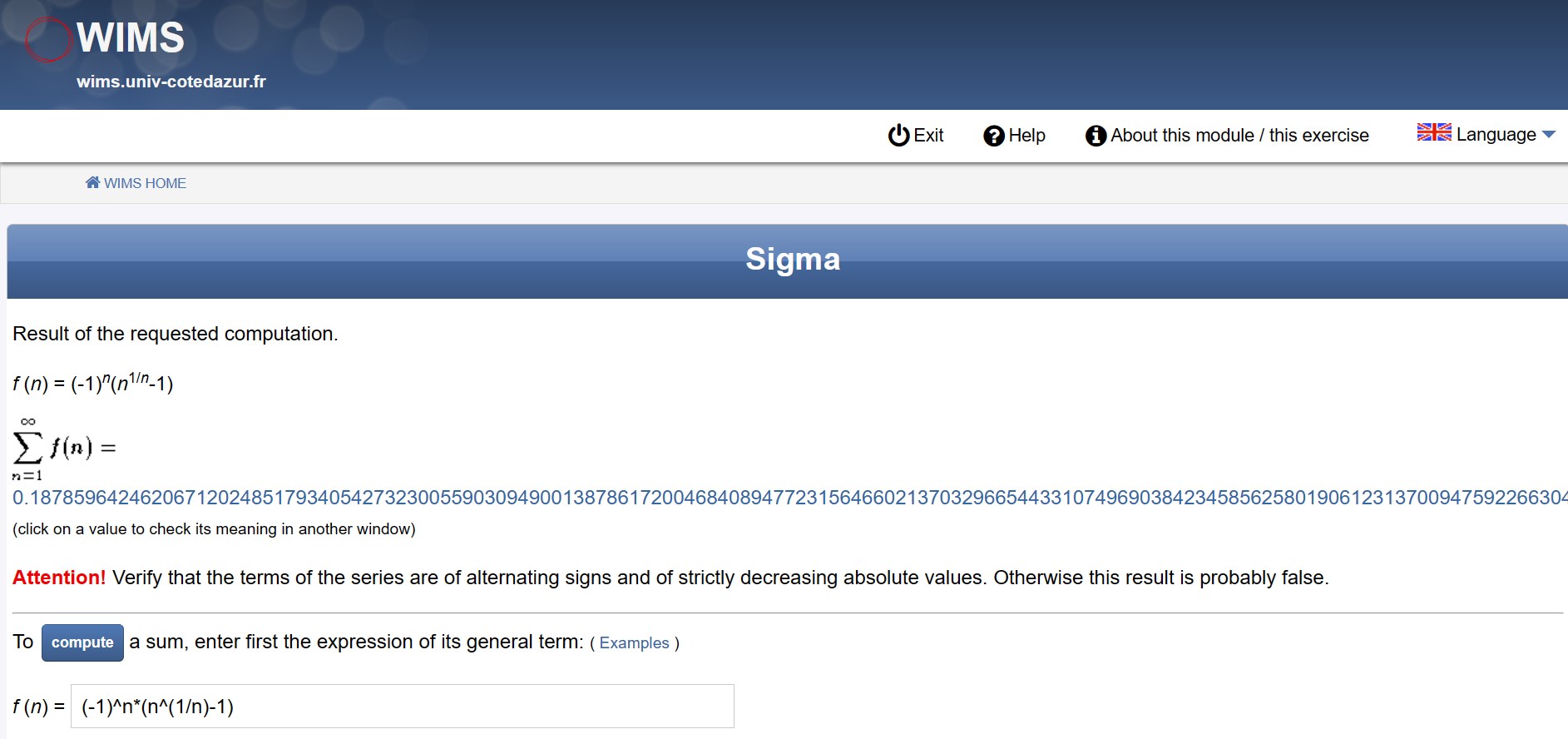 Sigma still can be found here.
5,000 digits of CMRB in September of 1999 in 2 hours on a 350 MHz PentiumII,133 MHz 64 MB of RAM using the simple PARI commands \p 5000;sumalt(n=1,((-1)^n*(n^(1/n)-1))), after allocating enough memory.
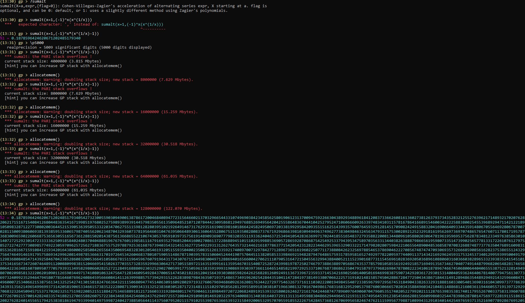
To beat that, it was done on July 4, 2022, in 1 second on the 5.5 GHz CMRBSC 3 with 4800MHz 64 GB of RAM by Newton's method using Convergence acceleration of alternating series. Henri Cohen, Fernando Rodriguez Villegas, Don Zagier acceleration "Algorithm 1" to at least 5000 decimals. (* Newer loop with Newton interior. *)
here.
Also,
here,
I did it using an i9-14900K, overclocked, with 64GB of 6400MHz RAM. I used my own program. Processor and actual time were 0.796875 and 0.8710556 s, respectively.
6,995 accurate digits of CMRB were computed on June 10-11, 2003, over a period, of 10 hours, on a 450 MHz P3 with an available 512 MB RAM,
To beat that, it was done in <2.5 seconds on the MRBCSC 3 on July 7, 2022 (more than 14,400 times as fast!)
documentation here
To beat that, it was done in <1. 684 seconds on April 10, 2024 (more than 21,377 times as fast!). documentation [here][15]:
In[3]:= 10 hour*3600 seconds/hour/(1.684 seconds)

Out[3]= 21377.7
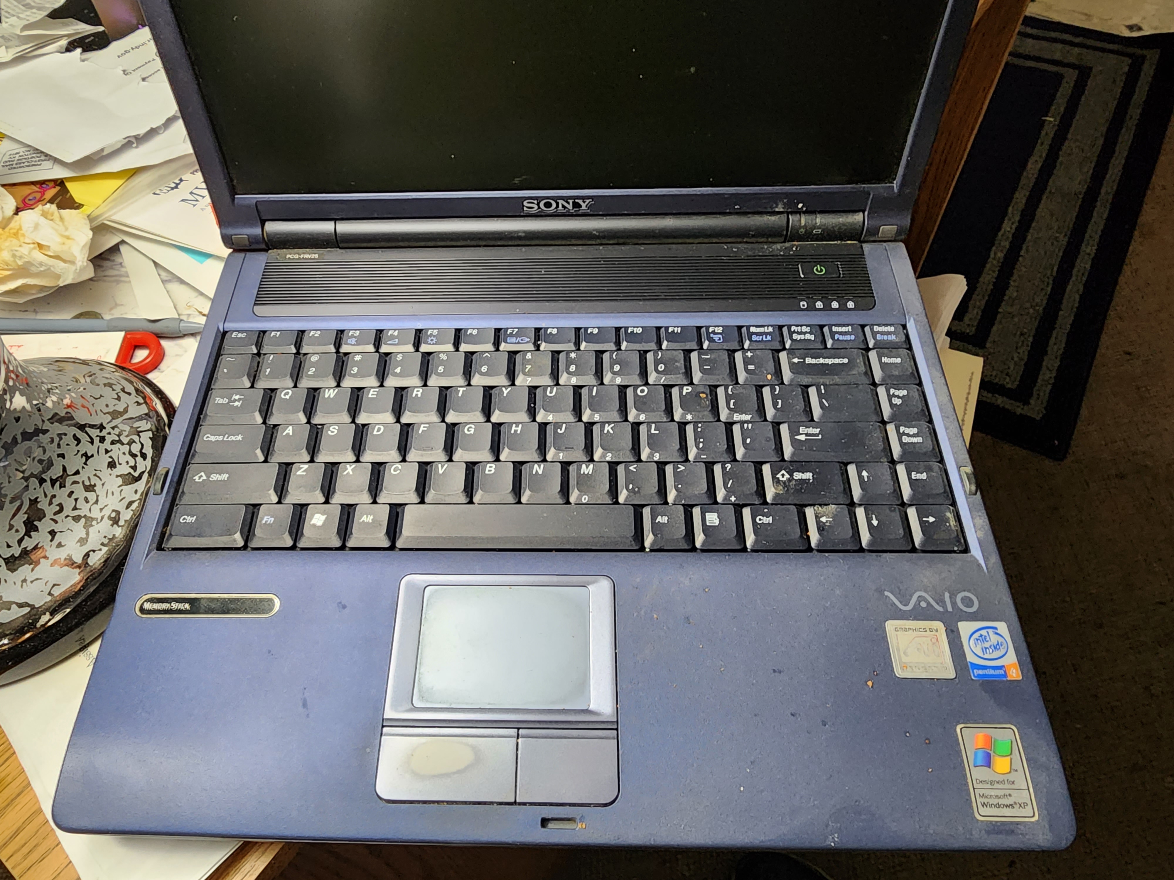
8000 digits of CMRB completed, using a Sony Vaio P4 2.66 GHz laptop computer with 960 MB of available RAM, at 2:04 PM 3/25/2004,
11,000 digits of CMRB> on March 01, 2006, with a 3 GHz PD with 2 GB RAM available calculated.
 40 000 digits of CMRB in 33 hours and 26 min via my program written in Mathematica 5.2 on Nov 24, 2006. The computation was run on a 32-bit Windows 3 GHz PD desktop computer using 3.25 GB of Ram.
The program was

    Block[{a, b = -1, c = -1 - d, d = (3 + Sqrt[8])^n,
      n = 131 Ceiling[40000/100], s = 0}, a[0] = 1;
     d = (d + 1/d)/2; For[m = 1, m < n, a[m] = (1 + m)^(1/(1 + m)); m++];
     For[k = 0, k < n, c = b - c;
      b = b (k + n) (k - n)/((k + 1/2) (k + 1)); s = s + c*a[k]; k++];
     N[1/2 - s/d, 40000]]
60,000 digits of CMRB on July 29, 2007, at 11:57 PM EST in 50.51 hours on a 2.6 GHz AMD Athlon with 64-bit Windows XP. The max memory used was 4.0 GB of RAM.
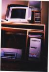
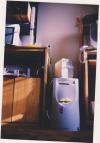
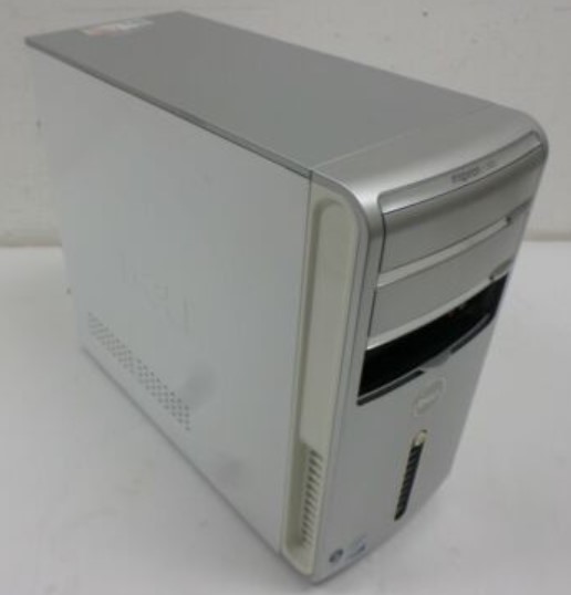
65,000 digits of CMRB in only 50.50 hours on a 2.66 GHz Core 2 Duo using 64-bit Windows XP on Aug 3, 2007, at 12:40 AM EST, The max memory used was 5.0 GB of RAM.
It looked similar to this stock image:
100,000 digits of CMRB on Aug 12, 2007, at 8:00 PM EST, were computed in 170 hours on a 2.66 GHz Core 2 Duo using 64-bit Windows XP. The max memory used was 11.3 GB of RAM. The typical daily record of memory used was 8.5 GB of RAM.
To beat that, on the 4th of July 2022, the same digits in 1/4 of an hour using the MRB constant supercomputer.
To beat that, on the 7th of July 2022, the same digits in 1/5 of an hour.
To beat that, on the 4th of April 2024, the same digits in 1/6 of an hour, using a pair of i9-14900Ks in the Wolfram Lightweight grid for V 11.3 (100,000% as fast as the first 100,000 run by a GHz Core 2 Duo!)
`To beat that, on the 8th of January 2025, I demonstrated all of its 131,000 nth roots computed to 100,000 digits, in parallel, in 1/69th of an hour (less than one minute)`
See less than one minute.
See one sixth hour hundred k.
150,000 digits of CMRB on Sep 23, 2007, at 11:00 AM EST. Computed in 330 hours on a 2.66 GHz Core 2 Duo using 64-bit Windows XP. The max memory used was 22 GB of RAM. The typical daily record of memory used was 17 GB of RAM.
200,000 digits of CMRB using Mathematica 5.2 on March 16, 2008, at 3:00 PM EST,. Found in 845 hours, on a 2.66 GHz Core 2 Duo using 64-bit Windows XP. The max memory used was 47 GB of RAM. The typical daily record of memory used was 28 GB of RAM.
300,000 digits of CMRB were destroyed (washed away by Hurricane Ike ) on September 13, 2008 sometime between 2:00 PM - 8:00 PM EST. Computed for a long  4015. Hours (23.899 weeks or 1.4454*10^7 seconds) on a 2.66 GHz Core 2 Duo using 64-bit Windows XP. The max memory used was 91 GB of RAM. The Mathematica 6.0 code is used as follows:

    Block[{$MaxExtraPrecision = 300000 + 8, a, b = -1, c = -1 - d,
     d = (3 + Sqrt[8])^n, n = 131 Ceiling[300000/100], s = 0}, a[0] = 1;
     d = (d + 1/d)/2; For[m = 1, m < n, a[m] = (1 + m)^(1/(1 + m)); m++];
     For[k = 0, k < n, c = b - c;
      b = b (k + n) (k - n)/((k + 1/2) (k + 1)); s = s + c*a[k]; k++];
     N[1/2 - s/d, 300000]]
225,000 digits of CMRB were started with a 2.66 GHz Core 2 Duo using 64-bit Windows XP on September 18, 2008. It was completed in 1072 hours.
250,000 digits were attempted but failed to be completed to a serious internal error that restarted the machine. The error occurred sometime on December 24, 2008, between 9:00 AM and 9:00 PM. The computation began on November 16, 2008, at 10:03 PM EST. The Max memory used was 60.5 GB.
250,000 digits of CMRB on Jan 29, 2009, 1:26:19 pm (UTC-0500) EST, with a multiple-step Mathematica command running on a dedicated 64-bit XP using 4 GB DDR2 RAM onboard and 36 GB virtual. The computation took only 333.102 hours. The digits are at http://marvinrayburns.com/250KMRB.txt. The computation is completely documented.
300000 digit search of CMRB was initiated using an i7 with 8.0 GB of DDR3 RAM onboard on Sun 28 Mar 2010 at 21:44:50 (UTC-0500) EST, but it failed due to hardware problems.
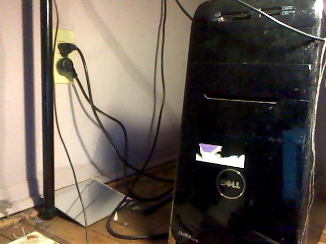
299,998 Digits of CMRB: The computation began Fri 13 Aug 2010 10:16:20 pm EDT and ended 2.23199*10^6 seconds later | Wednesday, September 8, 2010. using Mathematica 6.0 for Microsoft Windows (64-bit) (June 19, 2007), which averages 7.44 seconds per digit.using a Dell Studio XPS 8100 i7 860 @ 2.80 GHz with 8GB physical DDR3 RAM. Windows 7 reserved an additional 48.929 GB of virtual Ram.
300,000 digits to the right of the decimal point of CMRB from Sat 8 Oct 2011 23:50:40 to Sat 5 Nov 2011 19:53:42 (2.405*10^6 seconds later). This run was 0.5766 seconds per digit slower than the 299,998 digit computation even though it used 16 GB physical DDR3 RAM on the same machine. The working precision and accuracy goal combination were maximized for exactly 300,000 digits, and the result was automatically saved as a file instead of just being displayed on the front end. Windows reserved a total of 63 GB of working memory, of which 52 GB were recorded as being used. The 300,000 digits came from the Mathematica 7.0 command`
    Quit; DateString[]
    digits = 300000; str = OpenWrite[]; SetOptions[str,
    PageWidth -> 1000]; time = SessionTime[]; Write[str,
    NSum[(-1)^n*(n^(1/n) - 1), {n, \[Infinity]},
    WorkingPrecision -> digits + 3, AccuracyGoal -> digits,
    Method -> "AlternatingSigns"]]; timeused =
    SessionTime[] - time; here = Close[str]
    DateString[]
314159 digits of the constant took 3 tries due to hardware failure. Finishing on September 18, 2012, 314159 digits, taking 59 GB of RAM.  The digits came from the Mathematica 8.0.4 code`

    DateString[]
    NSum[(-1)^n*(n^(1/n) - 1), {n, \[Infinity]},
    WorkingPrecision -> 314169, Method -> "AlternatingSigns"] // Timing
    DateString[]
1,000,000 digits of CMRB for the first time in history in 18 days, 9 hours 11 minutes, 34.253417 seconds by Sam Noble of the Apple Advanced Computation Group.
1,048,576 digits of CMRB in a lightning-fast 76.4 hours, finishing on Dec 11, 2012, were scored by Dr. Richard Crandall, an Apple scientist and head of its advanced computational group. That was on a 2.93 GHz 8-core Nehalem,  1066 MHz, PC3-8500 DDR3 ECC RAM.

    To beat that, in Aug of 2018, 1,004,993 digits in 53.5 hours 34 hours computation time (from the timing command) with 10 DDR4 RAM (of up to 3000 MHz) supported processor cores overclocked up to 4.7 GHz! Search this post for "53.5" for documentation.

    To beat that, on Sept 21, 2018: 1,004,993 digits in 50.37 hours of absolute time and 35.4 hours of computation time (from the timing command) with 18  (DDR3 and DDR4) processor cores!  Search this post for "50.37 hours" for documentation.**

    To beat that, on May 11, 2019, over 1,004,993 digits in 45.5 hours of absolute time and only 32.5 hours of computation time, using 28 kernels on 18 DDR4 RAM (of up to 3200 MHz) supported cores overclocked up to  5.1 GHz  Search 'Documented in the attached ":3 fastest computers together 3.nb." '  for the post that has the attached documenting notebook.

    To beat that, over 1,004,993 correct digits in 44 hours of absolute time and 35.4206 hours of computation time on 10/19/20, using 3/4 of the MRB constant supercomputer 2 -- see https://www.wolframcloud.com/obj/bmmmburns/Published/44%20hour%20million.nb  for documentation.

    To beat that, a 1,004,993 correct digits computation in 36.7 hours of absolute time and only 26.4 hours of computation time on Sun 15 May 2022 at 06:10:50, using 3/4  of the MRB constant supercomputer 3. Ram Speed was 4800MHz, and all 30 cores were clocked at up to 5.2 GHz.


    To beat that, a 1,004,993 correct digits computation in 31.2319  hours of absolute time and 16.579  hours of computation time from the Timing[] command using 3/4 of the MRB constant supercomputer 4, finishing Dec 5, 2022. Ram Speed was 5200MHz, and all of the 24 performance cores were clocked at up to 5.95 GHz, plus 32 efficiency cores running slower. using 24 kernels on the Wolfram Lightweight grid over an i-12900k, 12900KS, and 13900K.
    To beat that, a 1,004,993 correct digits computation in 30. hours of absolute time on Marh 21, 2024.
    To beat that, a 1,004,993 correct digits computation in 27. hours
The 27-hour million-digit computation is found here <-Big notebook
see also 30 hour million
36.7 hours million notebook
31.2319 hours million
A little over 1,200,000 digits, previously, of CMRB in 11 days, 21 hours, 17 minutes, and 41 seconds (I finished on March 31, 2013, using a six-core Intel(R) Core(TM) i7-3930K CPU @ 3.20 GHz. see https://www.wolframcloud.com/obj/bmmmburns/Published/36%20hour%20million.nb
for details.
2,000,000 or more digit computation of CMRB on May 17, 2013, using only around 10GB of RAM. It took 37 days 5 hours, 6 minutes 47.1870579 seconds. using a six-core Intel(R) Core(TM) i7-3930K CPU @ 3.20 GHz.
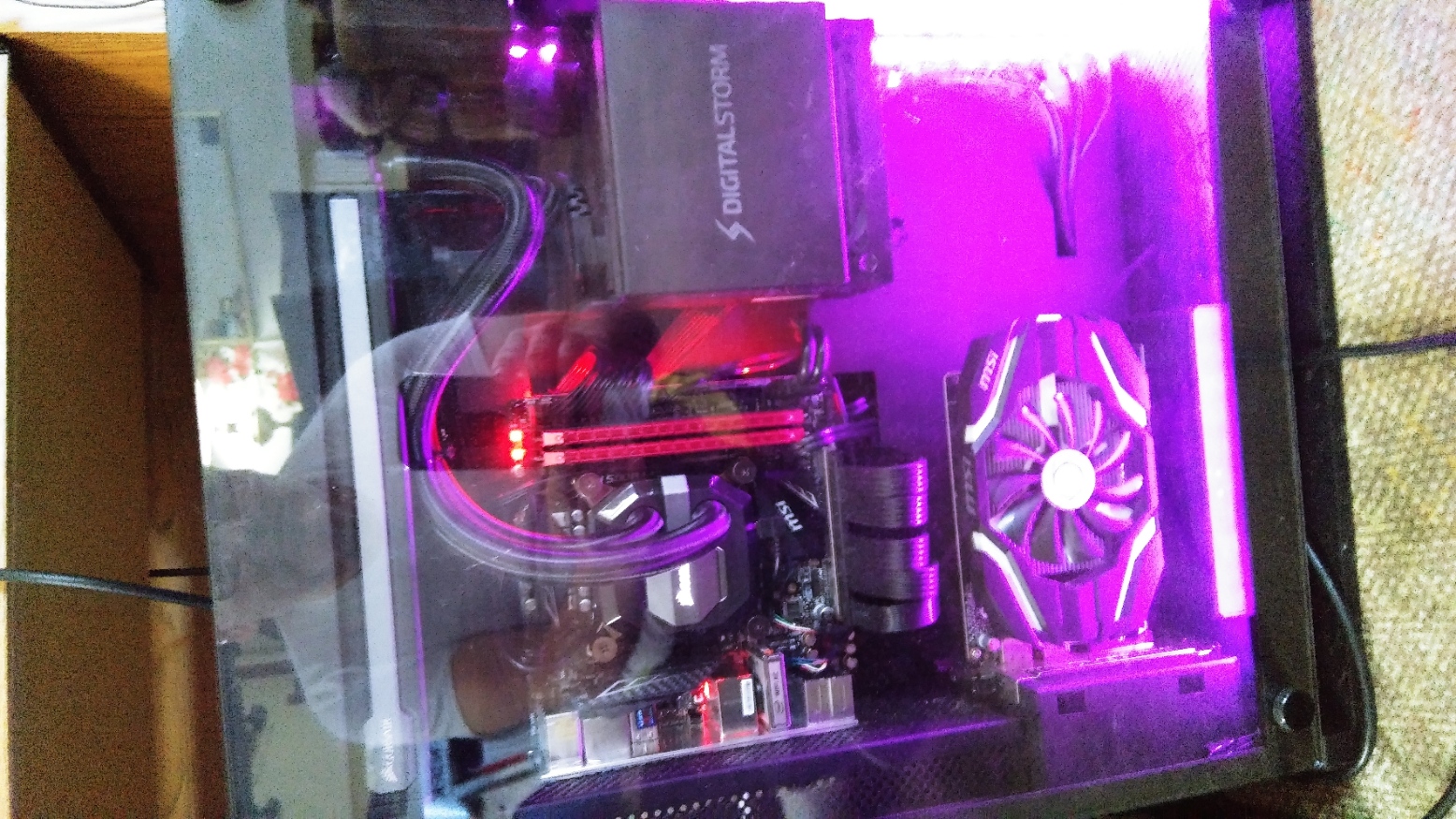
3,014,991 digits of CMRB, world record computation of **C**<sub>*MRB*</sub> was finished on Sun 21 Sep 2014 at 18:35:06. It took one month 27 days, 2 hours 45 minutes 15 seconds. The processor time from the 3,000,000+ digit computation was 22 days.The 3,014,991 digits of **C**<sub>*MRB*</sub> with Mathematica 10.0. using Burns' new version of Richard Crandall's code in the attached 3M.nb, optimized for my platform and large computations. Also, a six-core Intel(R) Core(TM) i7-3930K CPU @ 3.20 GHz with 64 GB of RAM, of which only 16 GB was used. Can you beat it (in more digits, less memory used, or less time taken)? This confirms that my previous "2,000,000 or more digit computation" was accurate to 2,009,993 digits. they were used to check the first several digits of this computation. See attached 3M.nb for the full code and digits.
 Over 4 million digits of CMRB were finished on Wed 16 Jan 2019, 19:55:20.
It took four years of continuous tries. This successful run took 65.13 days absolute time, with a processor time of 25.17 days, on a 3.7 GHz overclocked up to 4.7 GHz on all cores Intel 6 core computer with 3000 MHz RAM. According to this computation, the previous record, 3,000,000+ digit computation, was accurate to 3,014,871 decimals, as this computation used my algorithm for computing n^(1/n) as found in chapter 3 in the paper at
Over 4 million digits of CMRB were finished on Wed 16 Jan 2019, 19:55:20.
It took four years of continuous tries. This successful run took 65.13 days absolute time, with a processor time of 25.17 days, on a 3.7 GHz overclocked up to 4.7 GHz on all cores Intel 6 core computer with 3000 MHz RAM. According to this computation, the previous record, 3,000,000+ digit computation, was accurate to 3,014,871 decimals, as this computation used my algorithm for computing n^(1/n) as found in chapter 3 in the paper at
https://www.sciencedirect.com/science/article/pii/0898122189900242 and the 3 million+ computation used Crandall's algorithm. Both algorithms outperform Newton's method per calculation and iteration.


Example use of M R Burns' algorithm to compute 123456789^(1/123456789) 10,000,000 digits:

ClearSystemCache[]; n = 123456789;
(*n is the n in n^(1/n)*)
x = N[n^(1/n),100];
(*x starts out as a relatively small precision approximation to n^(1/n)*)
pc = Precision[x]; pr = 10000000;
(*pr is the desired precision of your n^(1/n)*)
Print[t0 = Timing[While[pc < pr, pc = Min[4 pc, pr];
x = SetPrecision[x, pc];
y = x^n; z = (n - y)/y;
t = 2 n - 1; t2 = t^2;
x = x*(1 + SetPrecision[4.5, pc] (n - 1)/t2 + (n + 1) z/(2 n t)
- SetPrecision[13.5, pc] n (n - 1)/(3 n t2 + t^3 z))];
(*You get a much faster version of N[n^(1/n),pr]*)
N[n - x^n, 10]](*The error*)];
ClearSystemCache[]; n = 123456789; Print[t1 = Timing[N[n - N[n^(1/n), pr]^n, 10]]]

 Gives

  {25.5469,0.*10^-9999984}

  {101.359,0.*10^-9999984}


  More information is available upon request.
More than 5 million digits of CMRB were found on Fri 19 Jul 2019, 18:49:02; methods are described in the reply below, which begins with "Attempts at a 5,000,000 digit calculation ." For this 5 million digit calculation of **C**<sub>*MRB*</sub> using the 3 node MRB supercomputer: processor time was 40 days. And the actual time was 64 days. That is in less absolute time than the 4-million-digit computation, which used just one node.
Six million digits of CMRB after eight tries in 19 months. (Search "8/24/2019 It's time for more digits!" below.) finishing on Tue, 30 Mar 2021, at 22:02:49 in 160 days.
    The MRB constant supercomputer 2 said the following:
    Finished on Tue 30 Mar 2021, 22:02:49. computation and absolute time were
    5.28815859375*10^6 and 1.38935720536301*10^7 s. respectively
    Enter MRB1 to print 6029991 digits. The error from a 5,000,000 or more-digit calculation that used a different method is
    0.*10^-5024993.

That means that the 5,000,000-digit computation Was accurate to 5024993 decimals!!!
5,609,880, verified by two distinct algorithms for x^(1/x), digits of CMRB on Thu 4 Mar 2021 at 08:03:45. The 5,500,000+ digit computation using a totally different method showed that many decimals are in common with the 6,000,000+ digit computation in 160.805 days.
6,500,000 digits of CMRB on my second try,
Successful code was:
In[2]:= Needs["SubKernels`LocalKernels`"]
Block[{$mathkernel = $mathkernel <> " -threadpriority=2"},
 LaunchKernels[]]

Out[3]= {"KernelObject"[1, "local"], "KernelObject"[2, "local"],
 "KernelObject"[3, "local"], "KernelObject"[4, "local"],
 "KernelObject"[5, "local"], "KernelObject"[6, "local"],
 "KernelObject"[7, "local"], "KernelObject"[8, "local"],
 "KernelObject"[9, "local"], "KernelObject"[10, "local"]}

In[4]:= Print["Start time is ", ds = DateString[], "."];
prec = 6500000;
(**Number of required decimals.*.*)ClearSystemCache[];
T0 = SessionTime[];
expM[pre_] :=
  Module[{a, d, s, k, bb, c, end, iprec, xvals, x, pc, cores = 16(*=4*
    number of physical cores*), tsize = 2^7, chunksize, start = 1, ll,
     ctab, pr = Floor[1.005 pre]}, chunksize = cores*tsize;
   n = Floor[1.32 pr];
   end = Ceiling[n/chunksize];
   Print["Iterations required: ", n];
   Print["Will give ", end,
    " time estimates, each more accurate than the previous."];
   Print["Will stop at ", end*chunksize,
    " iterations to ensure precsion of around ", pr,
    " decimal places."]; d = ChebyshevT[n, 3];
   {b, c, s} = {SetPrecision[-1, 1.1*n], -d, 0};
   iprec = Ceiling[pr/396288];
   Do[xvals = Flatten[Parallelize[Table[Table[ll = start + j*tsize + l;
         x = N[E^(Log[ll]/(ll)), iprec];
         pc = iprec;
         While[pc < pr/65536, pc = Min[3 pc, pr/65536];
          x = SetPrecision[x, pc];
          y = x^ll - ll;
          x = x (1 - 2 y/((ll + 1) y + 2 ll ll));];
         (**N[Exp[Log[ll]/ll],pr/99072]**)
         x = SetPrecision[x, pr/16384];
         xll = x^ll; z = (ll - xll)/xll;
         t = 2 ll - 1; t2 = t^2;
         x =
          x*(1 + SetPrecision[4.5, pr/16384] (ll - 1)/
               t2 + (ll + 1) z/(2 ll t) -
             SetPrecision[13.5,
               pr/16384] ll (ll - 1) 1/(3 ll t2 + t^3 z));(*N[Exp[Log[
         ll]/ll],pr/4096]*)x = SetPrecision[x, pr/4096];
         xll = x^ll; z = (ll - xll)/xll;
         t = 2 ll - 1; t2 = t^2;
         x =
          x*(1 + SetPrecision[4.5, pr/4096] (ll - 1)/
               t2 + (ll + 1) z/(2 ll t) -
             SetPrecision[13.5,
               pr/4096] ll (ll - 1) 1/(3 ll t2 + t^3 z));(*N[Exp[Log[
         ll]/ll],pr/4096]*)x = SetPrecision[x, pr/1024];
         xll = x^ll; z = (ll - xll)/xll;
         t = 2 ll - 1; t2 = t^2;
         x =
          x*(1 + SetPrecision[4.5, pr/1024] (ll - 1)/
               t2 + (ll + 1) z/(2 ll t) -
             SetPrecision[13.5,
               pr/1024] ll (ll - 1) 1/(3 ll t2 + t^3 z));(*N[Exp[Log[
         ll]/ll],pr/1024]*)x = SetPrecision[x, pr/256];
         xll = x^ll; z = (ll - xll)/xll;
         t = 2 ll - 1; t2 = t^2;
         x =
          x*(1 + SetPrecision[4.5, pr/256] (ll - 1)/
               t2 + (ll + 1) z/(2 ll t) -
             SetPrecision[13.5,
               pr/256] ll (ll - 1) 1/(3 ll t2 + t^3 z));(*N[Exp[Log[
         ll]/ll],pr/256]*)x = SetPrecision[x, pr/64];
         xll = x^ll; z = (ll - xll)/xll;
         t = 2 ll - 1; t2 = t^2;
         x =
          x*(1 + SetPrecision[4.5, pr/64] (ll - 1)/
               t2 + (ll + 1) z/(2 ll t) -
             SetPrecision[13.5,
               pr/64] ll (ll - 1) 1/(3 ll t2 + t^3 z));(**N[Exp[Log[
         ll]/ll],pr/64]**)x = SetPrecision[x, pr/16];
         xll = x^ll; z = (ll - xll)/xll;
         t = 2 ll - 1; t2 = t^2;
         x =
          x*(1 + SetPrecision[4.5, pr/16] (ll - 1)/
               t2 + (ll + 1) z/(2 ll t) -
             SetPrecision[13.5,
               pr/16] ll (ll - 1) 1/(3 ll t2 + t^3 z));(**N[Exp[Log[
         ll]/ll],pr/16]**)x = SetPrecision[x, pr/4];
         xll = x^ll; z = (ll - xll)/xll;
         t = 2 ll - 1; t2 = t^2;
         x =
          x*(1 + SetPrecision[4.5, pr/4] (ll - 1)/
               t2 + (ll + 1) z/(2 ll t) -
             SetPrecision[13.5,
               pr/4] ll (ll - 1) 1/(3 ll t2 + t^3 z));(**N[Exp[Log[
         ll]/ll],pr/4]**)x = SetPrecision[x, pr];
         xll = x^ll; z = (ll - xll)/xll;
         t = 2 ll - 1; t2 = t^2;
         x =
          x*(1 + SetPrecision[4.5, pr] (ll - 1)/
               t2 + (ll + 1) z/(2 ll t) -
             SetPrecision[13.5,
               pr] ll (ll - 1) 1/(3 ll t2 + t^3 z));(*N[Exp[Log[ll]/
         ll],pr]*)x, {l, 0, tsize - 1}], {j, 0, cores - 1}]]];
    ctab = ParallelTable[Table[c = b - c;
       ll = start + l - 2;
       b *= 2 (ll + n) (ll - n)/((ll + 1) (2 ll + 1));
       c, {l, chunksize}], Method -> "Automatic"];
    s += ctab.(xvals - 1);
    start += chunksize;
    st = SessionTime[] - T0; kc = k*chunksize;
    ti = (st)/(kc + 10^-4)*(n)/(3600)/(24);
    If[kc > 1,
     Print["As of  ", DateString[], " there were ", kc,
      " iterations done in ", N[st, 5], " seconds. That is ",
      N[kc/st, 5], " iterations/s. ", N[kc/(end*chunksize)*100, 7],
      "% complete.", " It should take ", N[ti, 6], " days or ",
      N[ti*24*3600, 4], "s, and finish ", DatePlus[ds, ti], "."]];
    Print[];, {k, 0, end - 1}];
   N[-s/d, pr]];
t2 = Timing[MRB1 = expM[prec];]; Print["Finished on ",
 DateString[], ". Proccessor and actual time were ", t2[[1]], " and ",
  SessionTime[] - T0, " s. respectively"];
Print["Enter MRB1 to print ",
 Floor[Precision[
   MRB1]], " digits. The error from a 5,000,000 or more digit \
calculation that used a different method is  "]; N[M6M - MRB1, 20]
The MRB constant supercomputer replied,
Finished on Wed 16 Mar 2022 02: 02: 10. computation and absolute time
were 6.26628*10^6 and 1.60264035419592*10^7s respectively Enter MRB1
to print 6532491 digits. The error from a 6, 000, 000 or more digit
the calculation that used a different method is
0.*10^-6029992.
"Computation time" 72.526 days.
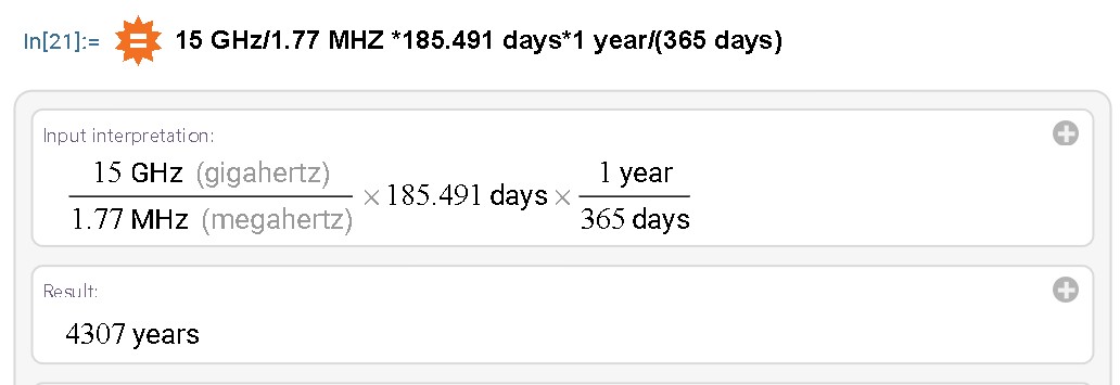
"Absolute time" 185.491 days.
It would have taken my first computer, a TRS-80 at least 4307 years with today's best mathematical algorithms.
15 GHz/1.77 MHZ 185.491 days1 year/(365 days)
It was instantly checked to 6,029,992 or so, digits by the program itself.
A 7-million-digit run using different number of digits of Exp[Log[ll]/ll] computed by each method, is in process, which will verify the residue of digits.


