Greeting. I am trying to replicate the results in the Table. 4 in this paper https://scispace.com/pdf/a-semi-analytical-state-space-approach-for-3d-transient-4l4ftso81u.pdf, "A semi-analytical state-space approach for 3D transient analysis of functionally graded material cylindrical shells". 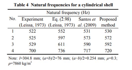
However, my code still gives wrong results and is far from the exact ones. I'm not sure whether the problems are in the code itself or elsewhere.
ClearAll["Global`*"]

(*1. INPUT PARAMETERS (Table 1)*)
l = 0.3048;   (*Length in m*)
Rm = 0.0762;   (*Radius in m*)
h = 0.000254;   (*Total thickness in m*)
a = Rm + h;  (*Outer radius in m*)
b = Rm;        (*Inner radius in m*)
(*Depth-to-length ratio*)(*Material Properties*)
\[Mu] = 0.3;
\[Rho] = 7860; (*Density in kg/m^3*)
Emod = 200*10^9; (*E in N/m^2*)
Gmod = Emod/(2*(1 + \[Mu]));
\[Lambda] = (Emod*\[Mu])/((1 + \[Mu])*(1 - 2*\[Mu]));
(*Stiffness coefficients for isotropic material*)
C11 = \[Lambda] + 2*Gmod;
C12 = \[Lambda];
C13 = \[Lambda];
C22 = C11;
C23 = \[Lambda];
C33 = C11;
C44 = Gmod;
C55 = Gmod;
C66 = Gmod;

(*Normalization parameters*)
c = Sqrt[C33/\[Rho]];

lr = 4;

(*2. DQM WEIGHTING MATRICES (Chebyshev-Gauss-Lobatto)*)
GetDQM[Npts_?NumericQ] :=
  Module[{xi, A, B, P},
   xi = Table[N[(1 - Cos[(i - 1) Pi/(Npts - 1)])/2], {i, 1, Npts}];
   A = Table[0, {Npts}, {Npts}];
   Do[P[i_] := Product[If[i == j, 1, xi[[i]] - xi[[j]]], {j, 1, Npts}];
    Do[If[i != j, A[[i, j]] = P[i]/((xi[[i]] - xi[[j]])*P[j])], {j, 1,
       Npts}];
    A[[i, i]] = -Sum[A[[i, j]], {j, 1, Npts}], {i, 1, Npts}];
   B = A.A;
   {N[A], N[B]}];
division[ri_, ro_, W_?NumericQ] :=
  Table[N[(ri/ro + ((2*m - 1)*(ro - ri))/(2*W*ro))], {m, 1, W}];
C11bar = C11/C33;
C12bar = C12/C33;
C13bar = C13/C33;
C22bar = C22/C33;
C23bar = C23/C33;
C44bar = C44/C33;
C55bar = C55/C33;
C66bar = C66/C33;
C33bar = 1;
(*Eta parameters from Eq.(19)*)
eta1 = C12bar/C11bar - 1;
eta2 = C22bar - C12bar^2/C11bar;
eta3 = C23bar - (C12bar*C13bar)/C11bar;
eta4 = C13bar^2/C11bar - C33bar;
eta5 = (C12bar*C13bar)/C11bar - (C23bar + C44bar);
(*3. REDUCED STATE SPACE MATRIX (Appendix A.1)*)
(*State vector:{u_1...u_N,sigma_2...sigma_N-1,v_2...v_N-1,tau_1...tau_\
N}*)
GetM[Omega_, j_, q_, N_?NumericQ, W1_, W2_] :=
  Module[{\[Rho]bar, R, dim, i2m, M},
   dim = 6*(N);
   R = division[b, a, lr][[q]];
   \[Rho]bar = 1;
   M = ConstantArray[0, {dim, dim}];
   i2m = 1;
   (*Sub-indices for state vector segments*)
   sIdx = 0; urIdx = N; utIdx = 2*(N); uzIdx = 3*(N); trzIdx = 4*(N);
   trtIdx = 5*(N);
   (*Subscript[d\[Sigma], r]/dr*)
   Do[Do[M[[sIdx + k, sIdx + k]] = eta1/R*i2m, {k, 2, N - 1}];
    Do[M[[sIdx + i,
       urIdx + k]] = -((a^2*C55bar)/l^2)*W1[[i, 1]]*W1[[1, k]] - (
        a^2*C55bar)/l^2*W1[[i, N]]*W1[[N, k]], {k, 2, N - 1}];
    M[[sIdx + i, urIdx + i]] += (\[Rho]bar*Omega^2 + eta2/R^2)*i2m;
    Do[M[[sIdx + k, utIdx + k]] = j*eta2/R^2*i2m, {k, 2, N - 1}];
    Do[M[[sIdx + i, uzIdx + k]] = a*eta3/(l*R)*W1[[i, k]], {k, 2,
      N - 1}];
    Do[M[[sIdx + i, trzIdx + k]] = -(a/l)*W1[[i, k]], {k, 2, N - 1}];
    Do[M[[sIdx + i, trtIdx + i]] = -(j/R)*i2m, {k, 2, N - 1}];, {i, 2,
      N - 1}];
   (*Subscript[du, r]/dr*)
   Do[Do[M[[urIdx + k, sIdx + k]] = 1/C11bar*i2m, {k, 2, N - 1}];
    Do[M[[urIdx + i, urIdx + i]] = -(C12bar/(R*C11bar))*i2m, {k, 2,
      N - 1}];
    Do[M[[urIdx + i, utIdx + i]] = -(j*C12bar/(R*C11bar))*i2m, {k, 2,
      N - 1}];
    Do[M[[urIdx + i, uzIdx + k]] = -(a*C13bar/(l*C11bar))*
       W1[[i, k]], {k, 2, N - 1}];, {i, 2, N - 1}];
   (*Subscript[du, \[Theta]]/dr*)
   Do[Do[M[[utIdx + i, urIdx + i]] = (j/R)*i2m, {k, 2, N - 1}];
    Do[M[[utIdx + i, utIdx + i]] = (1/R)*i2m, {k, 2, N - 1}];
    Do[M[[utIdx + i, trtIdx + i]] = (1/C66bar)*i2m, {k, 2,
      N - 1}];, {i, 2, N - 1}];
   (*Subscript[du, z]/dr*)
   Do[Do[M[[uzIdx + i, urIdx + k]] = -(a/l)*W1[[i, k]], {k, 2,
      N - 1}];
    Do[M[[uzIdx + i, trzIdx + i]] = (1/C55bar)*i2m, {k, 2,
      N - 1}];, {i, 2, N - 1}];
   (*Subscript[d\[Tau], rz]/dr*)
   Do[Do[M[[trzIdx + i, sIdx + k]] = -(a*C13bar/(l*C11bar))*
       W1[[i, k]], {k, 2, N - 1}];
    Do[M[[trzIdx + i, urIdx + k]] = -(a*eta3/(l*R))*W1[[i, k]], {k, 2,
       N - 1}];
    Do[M[[trzIdx + i, utIdx + k]] = -(j*a/(l*R))*(eta3 + C44bar)*
       W1[[i, k]], {k, 2, N - 1}];
    Do[M[[trzIdx + i,
       uzIdx + k]] = (a^2*eta4/(l^2))*
        W2[[i, k]] - (a^2*C13bar^2/(l^2*C11bar))*W1[[i, 1]]*
        W1[[1, k]] - (a^2*C13bar^2/(l^2*C11bar))*W1[[i, N]]*
        W1[[N, k]], {k, 2, N - 1}];
    M[[trzIdx + i,
      urIdx + i]] += (\[Rho]bar*Omega^2 + j^2*C44bar/R^2)*i2m;
    Do[M[[trzIdx + i, trzIdx + i]] = -(1/R)*i2m, {k, 2, N - 1}];, {i,
     2, N - 1}];
   (*Subscript[d\[Tau], r\[Theta]]/dr*)
   Do[Do[M[[trtIdx + i, sIdx + i]] = (j*C12bar/(R*C11bar))*i2m, {k, 2,
       N - 1}];
    Do[M[[trtIdx + i, urIdx + i]] = (j*eta2/R^2)*i2m, {k, 2, N - 1}];
    Do[M[[trtIdx + i, utIdx + k]] = -(a^2*C44bar/l^2)*W2[[i, k]], {k,
      2, N - 1}];
    M[[trtIdx + i, utIdx + i]] += (\[Rho]bar*Omega^2 + j^2*eta2/R^2)*
      i2m;
    Do[M[[trtIdx + i, uzIdx + k]] = (a*j/(l*R))*(eta3 + C44bar)*
       W1[[i, k]], {k, 2, N - 1}];
    Do[M[[trtIdx + i, trtIdx + i]] = -(2/R)*i2m, {k, 2, N - 1}];, {i,
     2, N - 1}];
   M];
(*4. FREQUENCY SOLVER*)
GetFreq[Omega_?NumericQ, Npts_?NumericQ] :=
  Module[{W1, W2, S, Mi, subt, ss}, {W1, W2} = GetDQM[Npts];
   S = IdentityMatrix[6*Npts];
   Do[Mi = GetM[Omega, 5, k, Npts, W1, W2];
    S = MatrixExp[Mi*(h)/(lr*a)].S;, {k, 1, lr}];
   (*Partition for traction-free surface:Subscript[\[Sigma], r]=
   Subscript[\[Tau], rz]=Subscript[\[Tau], r\[Theta]]=0*)
   rowIdx =
    Join[Range[2, Npts - 1], Range[4 (Npts) + 2, 5 Npts - 1],
     Range[5 Npts + 2, 6 Npts - 1]];
   colIdx =
    Join[Range[Npts + 2, 2 Npts - 1], Range[2 Npts + 2, 3 Npts - 1],
     Range[3 Npts + 2, 4 Npts - 1]];
   subt = S[[rowIdx, colIdx]];
   ss = Det[subt]; ss];
(*5. OUTPUT RESULTS (N=15)*)
GetFreq[0.045, 15,5]
Nval = 15;
fscale = (1/(2 Pi*a))*Sqrt[C33/\[Rho]]
Do[guess = Range[500, 800, 10][[j]]/fscale;
  sol = w /.
    Last@FindMinimum[Log[Abs[GetFreq[w, Nval, j]]], {w, guess}];
  Print["Frequency for j = ", j]
   Print["Mode ", j, ": ", (sol)*fscale, " Hz"];, {j, 1, 6}];
Results:
12183.46984
0.04103921187

During evaluation of In[48]:= Frequency for j = 1
During evaluation of In[48]:= Mode 1: -0.0002906076168 Hz
During evaluation of In[48]:= FindMinimum::lstol: The line search decreased the step size to within the tolerance specified by AccuracyGoal and PrecisionGoal but was unable to find a sufficient decrease in the function. You may need more than MachinePrecision digits of working precision to meet these tolerances.
During evaluation of In[48]:= Frequency for j = 2
During evaluation of In[48]:= Mode 2: 0.0002546168015 Hz
During evaluation of In[48]:= Frequency for j = 3
During evaluation of In[48]:= Mode 3: -0.00004378307522 Hz
During evaluation of In[48]:= Frequency for j = 4
During evaluation of In[48]:= Mode 4: 0.0001423820262 Hz
During evaluation of In[48]:= Frequency for j = 5
During evaluation of In[48]:= Mode 5: 0.0002601605751 Hz
During evaluation of In[48]:= Frequency for j = 6
During evaluation of In[48]:= Mode 6: 0.0000456248529 Hz
During evaluation of In[79]:= FindRoot::lstol: The line search decreased the step size to within tolerance specified by AccuracyGoal and PrecisionGoal but was unable to find a sufficient decrease in the merit function. You may need more than MachinePrecision digits of working precision to meet these tolerances.
During evaluation of In[79]:= Frequency for j = 5
During evaluation of In[79]:= Mode 1: 0.00007144391358 Hz
During evaluation of In[79]:= FindRoot::lstol: The line search decreased the step size to within tolerance specified by AccuracyGoal and PrecisionGoal but was unable to find a sufficient decrease in the merit function. You may need more than MachinePrecision digits of working precision to meet these tolerances.
During evaluation of In[79]:= Frequency for j = 5
During evaluation of In[79]:= Mode 2: -0.0001566304623 Hz
How can this code generate more robust results that converge to the values in Table 4 of the paper in the link? Here are the relevant equations used in the code.
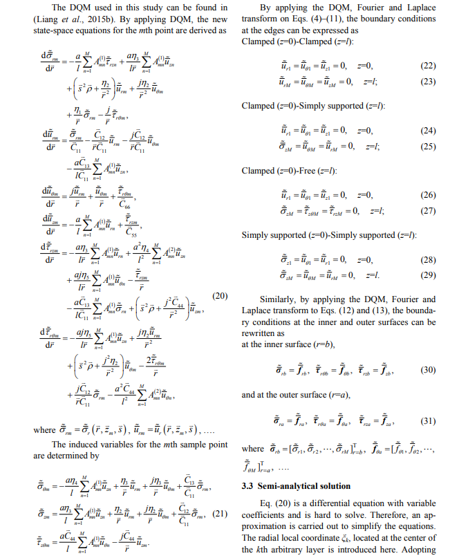
Eq. 20 is used besides Eqs.(22,23) for formulating the matrix H in Eq.33
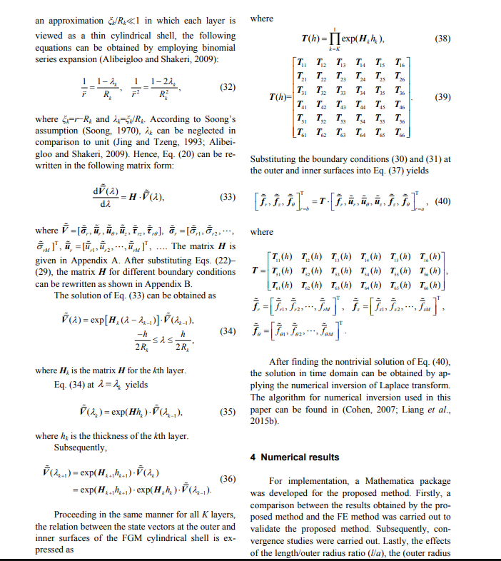
Matrix H is used in Eq.38 to obtain the transfer matrix T. Then, as we have a stress-free case as boundary conditions in the radial direction, Eq. 40 will be reduced into a 3X3 matrix, from which we obtain the roots after taking its determinant = 0.
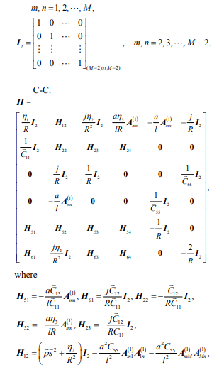
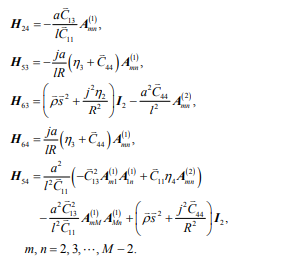
The elements of H matrix


