Re "0 can have any dimension":
First, we should agree, which I think we do, that your actual input to NDSolve[] in your first example is NDSolve[{y'[t] == {-y[t], 0}, y[0] == {1, 1}}, y, {t, 0, 1}]. The ODE is y'[t] == {-y[t], 0} and the IC is y[0] == {1, 1}. This is what I'm discussing, and if we don't agree, then we're talking past each other.
I'm not sure that 0 can have any dimension is really true. There is an operation called threading that can make scalars seem so (e.g. Solve[{x, y} == 1], which is broken down as x == 1 and y == 1 as if Thread[{x, y} == 1] were the input). In your example, the problem is that NDSolve[] performs a sort of de-threading of the input you give. Threading is not invertible, so NDSolve[] must be de-threading by making certain assumptions. In some circumstances, "making certain assumptions" is called a bug. You can file a bug report by using the menu command in Mathematica: Help > Give Feedback... which will take you to a webform for reporting bugs. See the Appendix below for more on de-threading.
Anyway, back to "0 can have any dimension": Why do you think that? Perhaps it is something I don't know. I've always understood that some functions will thread scalars in some circumstances. Not every function handles threading the same (see the case study in the Appendix for an example).
@David Trimas's "workaround" points out the problem with de-threading. His example feels like a red herring to me, but it's not irrelevant. I don't know when the de-threading was implemented. I didn't notice it until I looked into David's example. The proper workaround, I would suggest, is the following use of Indexed[], which I suppose de-threading was implemented to make unnecessary:
NDSolve[{
  y'[t] == -{1, 0}*{Indexed[y[t], 1], Indexed[y[t], 2]},
  y[0] == {1, 1}},
 y, {t, 0, 1}]
@khan ali has kindly pointed out how the DiagonalMatrix approach is different from, and not inconsistent with, the vector approach.
Here are a couple more, rather recherché, workarounds. The second is faster, but it's based on the assumption that once the ODE is evaluated numerically, it is never again evaluated symbolically in the call to NDSolve[].
times // ClearAll;
times[a : __?(VectorQ[#, NumericQ] &)] := Times[a];
NDSolve[{
  y'[t] == -times[{1, 0}, y[t]],
  y[0] == {1, 1}},
 y, {t, 0, 1}]

times // ClearAll;
times[a : __?(VectorQ[#, NumericQ] &)] := (times = Times)[a];
NDSolveValue[{
  y'[t] == -times[{1, 0}, y[t]],
  y[0] == {1, 1}},
 y, {t, 0, 1}]
You say that the ODE is the vector form of the differential equation. I disagree that {-y[t], 0} is a vector, which is why I defined above what the ODE is in my view. A vector in Mathematica is a list of scalars and not, say, a column matrix, as it sometimes is in math&science. If {-y[t], 0} is a vector, then -y[t] should be a scalar. But it is itself a vector. It might be that "0 can have any dimension" is supposed to explain why {-y[t], 0} can be a vector. I can interpret that only as {-y[t], 0} is the same as the vector -y[t]. I don't see how the outer List[] can be stripped away, even if 0 can have any dimension. And {-y[t]} is a
$1\times2$ matrix (tensor rank 2), not a vector. So y'[t], which is a 2-vector (tensor rank 1), cannot be equal to the matrix expression {-y[t]}; but if you de-thread {-y[t]} as {-1, -1} * y[t] when y[t] has the value of a numeric 2-vector {y1, y2}, then the de-threaded expression {-1, -1} * {y1, y2} evaluates to the 2-vector {-y1, -y2}.
In David's workaround, {-y[t], $MachineEpsilon*y[t]} is de-threaded and evaluated as a 2-vector as follows:
{-y[t], $MachineEpsilon * y[t]}     -->
  {-1, $MachineEpsilon} * y[t]      -->
  {-1, $MachineEpsilon} * {y1, y2}  -->
  {-y1, $MachineEpsilon * y2}
So the differential system being integrated in effect is
${y_1'(t)} = {-y_1(t)}$,
$y_2'(t) = 2^{-52} y_2(t)$,
where
y[t]
is represented by
$\big({y_1}(t)$,
${y_2}(t)\big)$.
In the OP's first example, {-y[t], 0} is not de-threaded because (I assume) the second element does not have a factor of y[t] literally present(!): y[t] appears only in the first element. This is the source of the failure of NDSolve[] in this case.
Appendix
What is de-threading? How does it arise in NDSolve[]?
It's my name for a partial inverse operation to Thread[]. One might thread at multiple levels when a expressions consists of nested lists. I'll stick to the simple case of a vector list. Then the basic idea is that if y = dethread[x], then Thread[y] === x; the converse need not be true.
To see how NDSolve[] processes the ODE (when successful), one can inspect the numerical function it creates for evaluating y'[t]. When it's unsuccessful, no numerical function is created, as in the case of the OP's first example. The function expression shows the formula used, in which we can see the de-threading. The symbol y stands for the value of y[t]. I've shown the dimensions NDSolve[] is using: {} denotes that t is a scalar; {n} denotes that the argument y and the result (for y') is a vector of length n.
checkODE[args___] := Module[{state},
   {state} = NDSolve`ProcessEquations[args];
   Grid[
    {#, state["NumericalFunction"]@#} & /@ {"FunctionExpression",
      "ArgumentDimensions", "ResultDimensions"}
    , Alignment -> Left, Spacings -> {1, Automatic}]
   ];

checkODE[ (* like David Trimas's ODE: y[t] in each component *)
 {y'[t] == {-1, -2, -3} y[t], y[0] == {1, 1, 1}}
 , y, {t, 0, 1}]
checkODE[ (* yet another workaround for the OP's problem *)
 {y'[t] == {-y[t], 2 (1 + y[t]) - 2 - 2 y[t]}, y[0] == {1, 1}}
 , y, {t, 0, 1}]
checkODE[ (* buggy!!! *)
 {y'[t] == -{t + 1, t + 2, t + y[t]}*y[t], y[0] == {1, 1, 1}}
 , y, {t, 0, 1}]
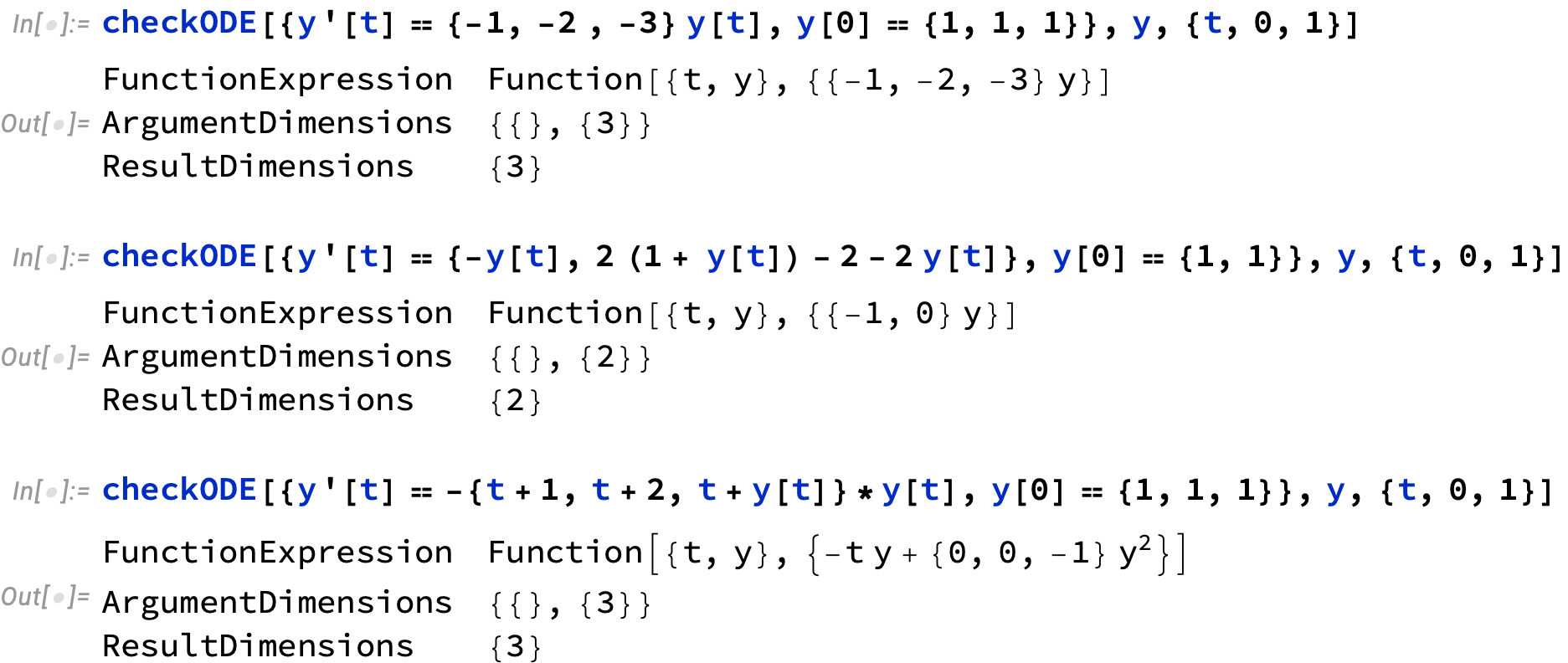
Note that the last example is a real bug. NDSolve[] produces a solution but the wrong one: The first two components in the wrong answer are identical since the function expression is missing part of each linear term:
-{t + 1, t + 2, t + y[t]}*y[t] - (* ODE's y'[t] *)
  (- t y + {0, 0, -1} y^2 /. y -> y[t]) // (* NumericalFunction's y' *)
 Simplify
(*  {-y[t], -2 y[t], 0}  <-- should be {0, 0, 0} *)
One might also question whether it is clear what the ODE y'[t] == -{t + 1, t + 2, t + y[t]}*y[t] is supposed to mean in the first place. I suppose a reasonable interpretation is that it represents the three independent 1D ODEs:
$$y'=-(t+1)y \,,\quad y' = -(t+2)y \,,\quad y'=-(ty+y^2)\,.$$
Case study: Solve is more forgiving than DSolve, which in turn is more forgiving than NDSolve
NDSolve[{{x'[t], y'[t]} == 0     , {x[0], y[0]} == 0},
 {x, y}, {t, 0, 1}] (* failure: NDSolve::underdet *)
NDSolve[{{x'[t], y'[t]} == {0, 0}, {x[0], y[0]} == 0},
 {x, y}, {t, 0, 1}] (* failure: NDSolve::ndnco *)
NDSolve[{{x'[t], y'[t]} == {0, 0}, {x[0], y[0]} == {0, 0}},
 {x, y}, {t, 0, 1}] (* success *)

DSolve[{{x'[t], y'[t]} == 0     , {x[0], y[0]} == 0},
 {x, y}, {t, 0, 1}] (* failure: DSolve::nolist *)
DSolve[{{x'[t], y'[t]} == {0, 0}, {x[0], y[0]} == 0},
 {x, y}, {t, 0, 1}] (* success *)
DSolve[{{x'[t], y'[t]} == {0, 0}, {x[0], y[0]} == {0, 0}},
 {x, y}, {t, 0, 1}] (* success *)

Solve[{{x'[t], y'[t]} == 0     , {x[0], y[0]} == 0     }] (* success *)
Solve[{{x'[t], y'[t]} == {0, 0}, {x[0], y[0]} == 0     }] (* success *)
Solve[{{x'[t], y'[t]} == {0, 0}, {x[0], y[0]} == {0, 0}}] (* success *)
I'm not sure this ordering is always the case, but Solve[] is usually more robust than either of NDSolve[] or DSolve[].


