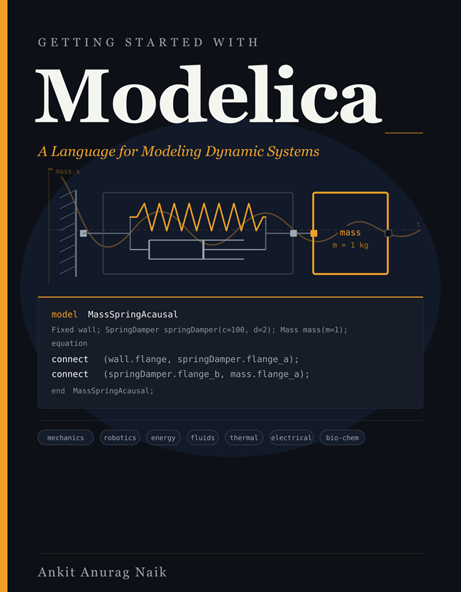
I'm excited to share that my new book, Getting Started with Modelica, is now available on Amazon.
Amazon Page
Who is it for?
Engineers and students taking their first serious steps with Modelica. No prior Modelica experience required. If you are already using System Modeler for drag-and-drop modeling and want to understand what is happening under the hood, or start writing your own textual models, this book is for you.
What does it cover?
The essentials you need to go from zero to writing and reading Modelica code. Acausal modeling and connectors, the Modelica Standard Library, inheritance, events, arrays, functions, records, solver internals, and FMI. By the end, you will be able to read code from the Modelica Standard Library, write your own models, and diagnose common problems independently.
Why does it matter in the age of LLMs?
LLMs can generate Modelica. But spotting when it's wrong takes a human who understands the language. This book builds that understanding.
Selected Figures from the Book
1. Why Modelica? — multi-domain systems
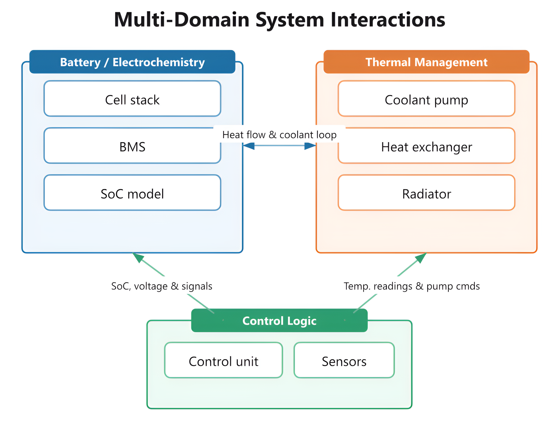
Multi-domain system: battery, fluid/thermal, and control logic coupled in a single model.
Real systems rarely live in one physical domain. An EV battery's state-of-charge depends on its temperature, which depends on the coolant loop, which depends on the control logic that watches both. Modelica lets you describe each domain in its own language — electrical, thermal, fluid, control — and assemble them in one simulation, with the coupling at the boundaries handled by the connectors.
2. Causal vs. acausal modeling
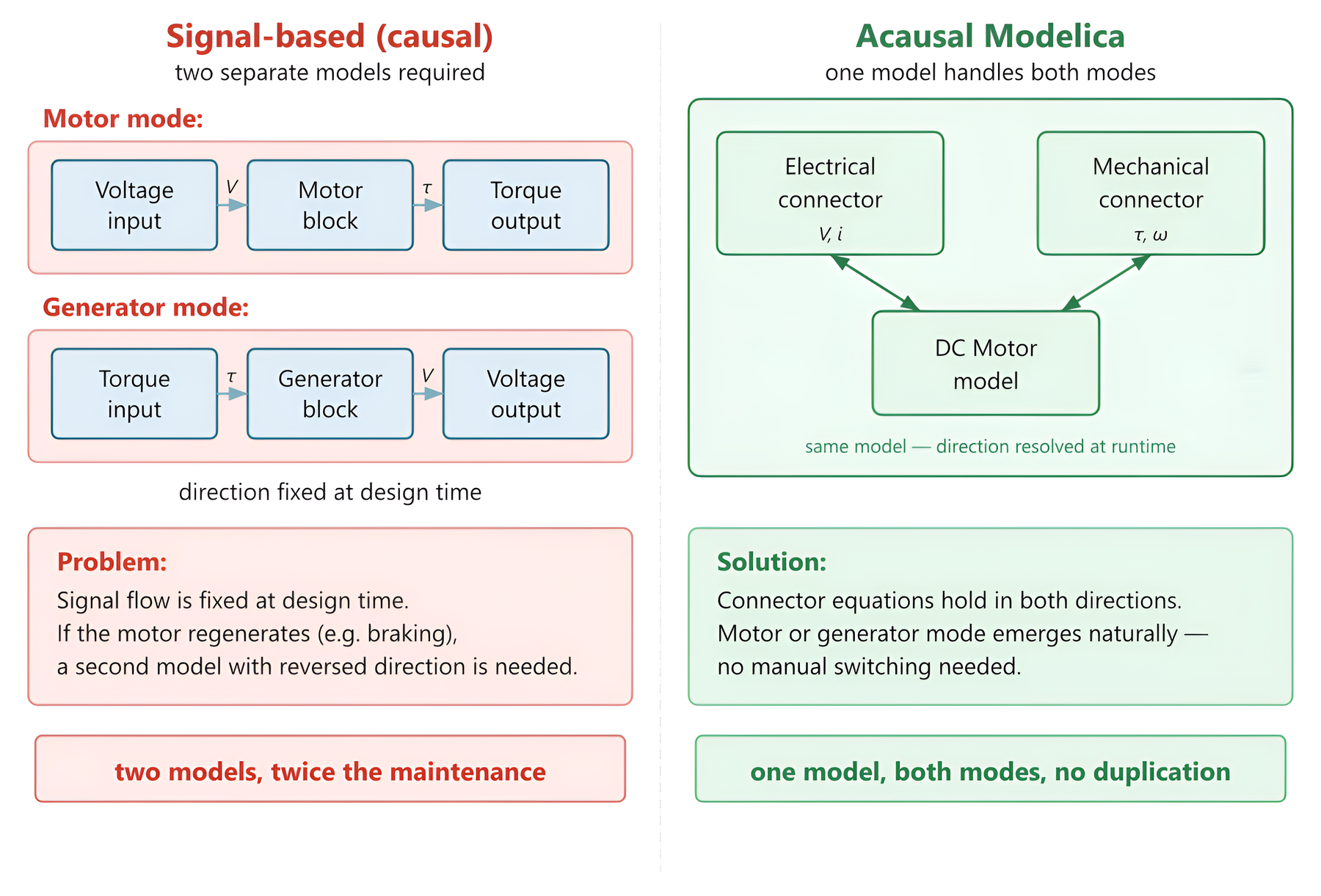
Causal approach requires two separate models; one acausal Modelica model handles both naturally.
This is the single image that captures what makes Modelica different. A signal-based tool freezes the direction of information flow at design time, so a motor and a generator are two different models even though the physics is identical. In Modelica you write the equations once; the compiler decides at solve time whether torque is the input or the output, based on how the component is connected. The same DC machine model handles motoring and regeneration — no manual switching, no duplication.
3. Hybrid simulation: continuous + discrete
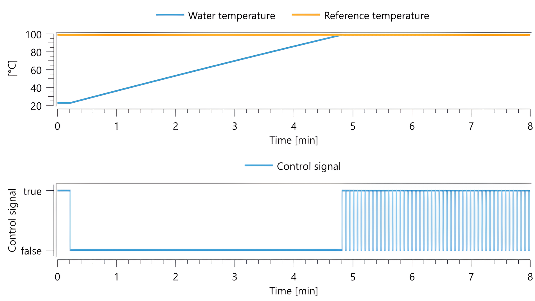
Thermostat simulation: continuous temperature dynamics and discrete switching in one run.
Real engineering systems mix smooth continuous physics with sharp discrete events: a valve opens, a relay clicks, a controller switches mode. Modelica handles both natively — the solver pauses cleanly at each event, applies any state changes, and resumes. Here the water heats up continuously while a discrete control signal toggles the heater on and off around the setpoint, all inside the same simulation.
4. The bouncing ball — events done right
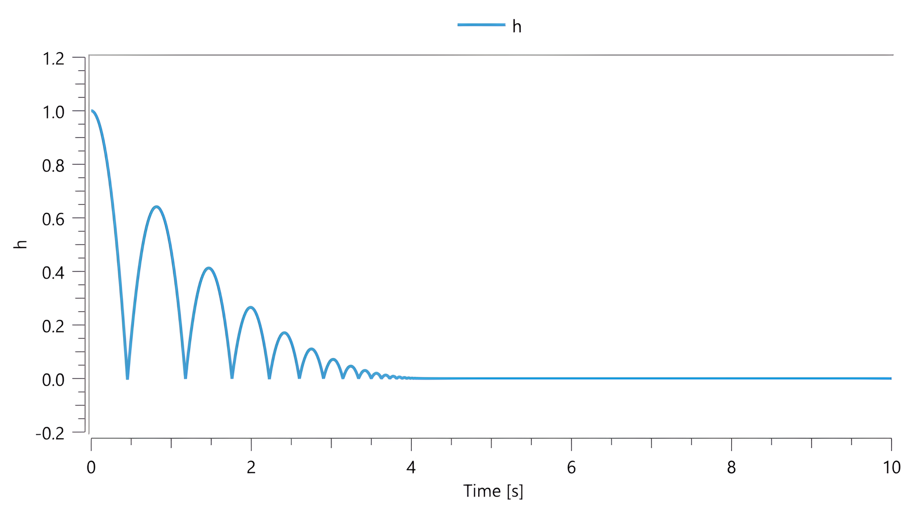
Bouncing ball height: each arc lower than the last as energy is lost to the restitution coefficient.
The bouncing ball is the canonical event-handling test in any simulation language. The solver follows ballistic flight, detects each ground impact as a zero-crossing, reinitializes the velocity through Modelica's reinit() operator, and continues. The energy loss per bounce is captured in a single coefficient of restitution — no special-case code, no workarounds.
5. Why event handling matters
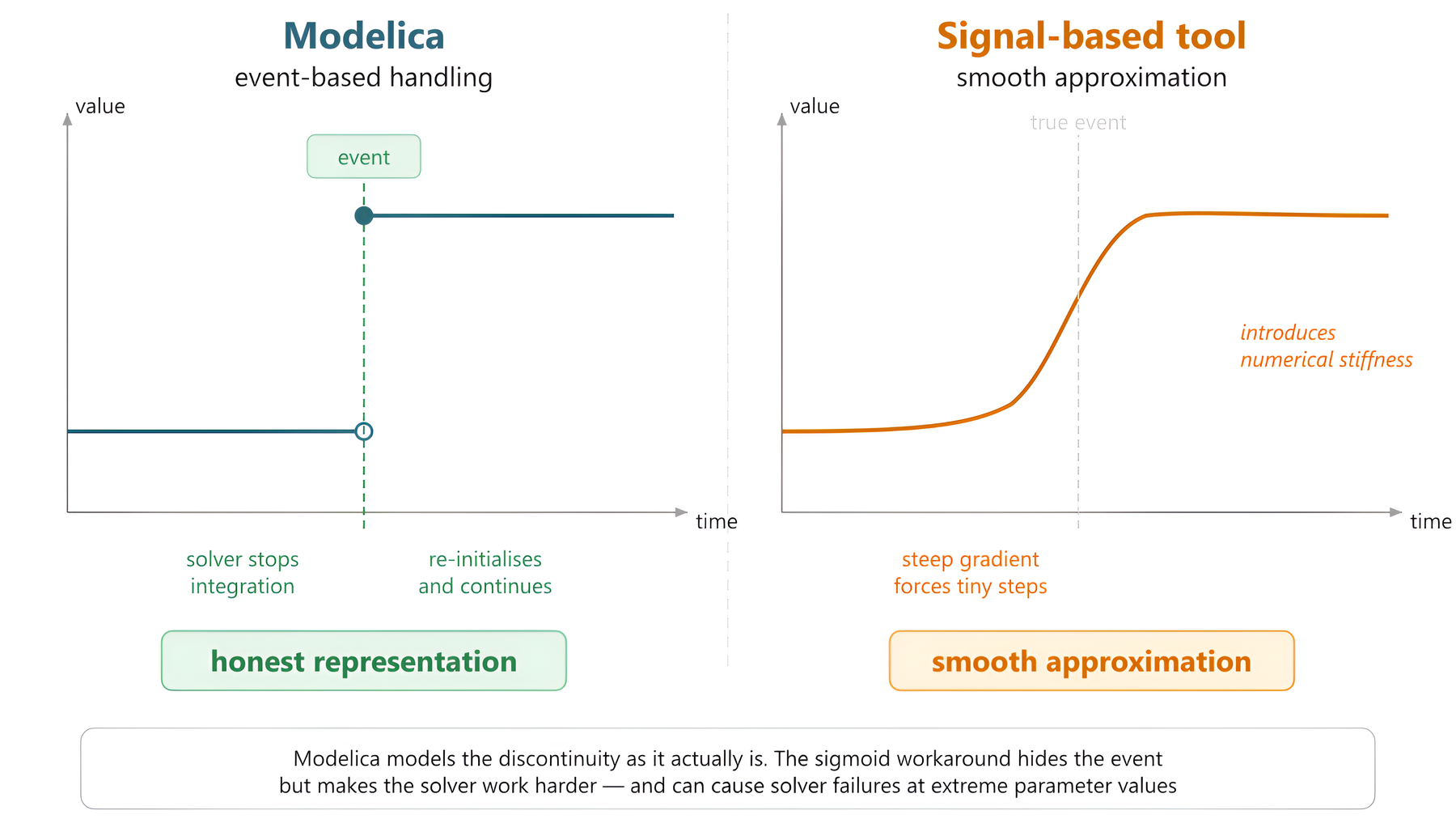
Modelica stops at discontinuities and handles them explicitly; signal-based tools approximate them as steep smooth curves.
A common workaround in signal-based tools is to model a switch as a steep sigmoid. It looks tidy, but the steep gradient forces the integrator into tiny time steps and can cause solver failures at extreme parameter values. Modelica represents the discontinuity honestly — the solver stops, re-initializes, and continues — which is both faster and numerically robust.
6. Inheritance in the Modelica Standard Library
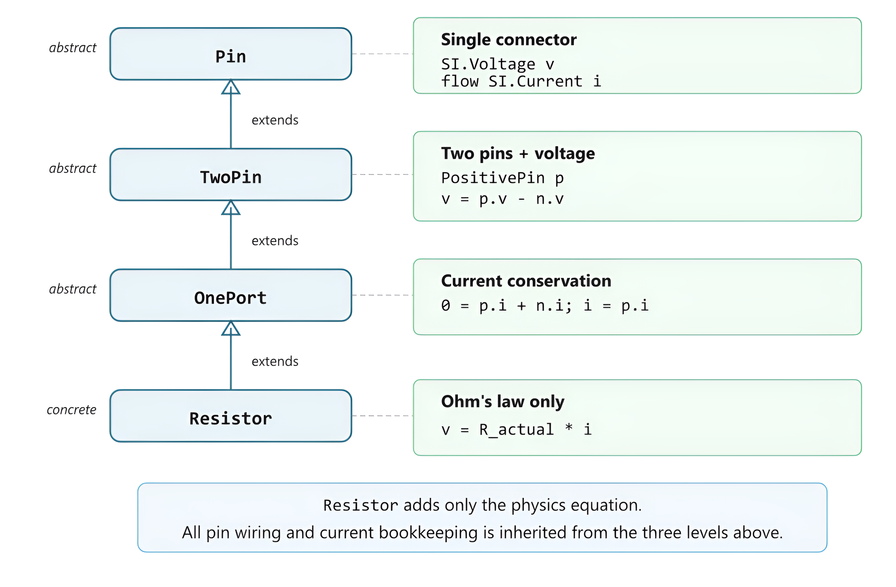
MSL Resistor inheritance chain: each level adds exactly one thing (connector, voltage difference, current conservation, Ohm's law).
The Modelica Standard Library is built on disciplined object-oriented design. The Resistor doesn't define its pins, voltage difference, or current bookkeeping — those are inherited from three abstract layers above it (Pin, TwoPin, OnePort). The concrete component contributes one equation: v = R*i. This is why MSL components compose so cleanly across thousands of models and dozens of domains.
7. A real engineering example — heated pipe
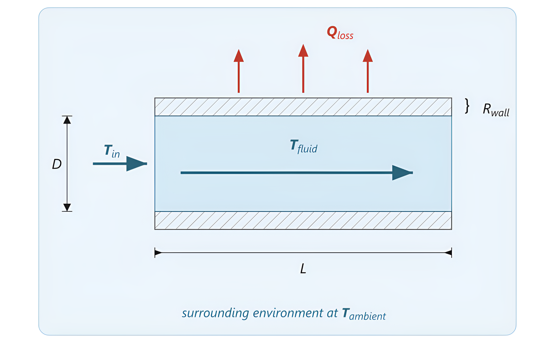
The pipe system: fluid enters at Tin, loses heat through wall resistance Rwall to ambient T_ambient.
Chapter 10 builds a heated-pipe model from scratch over four stages, introducing one new concept at each step — geometry parameters, fluid properties, the energy balance, then heat loss to the environment. This sketch is the physical picture the model is built from. The pedagogy: start from a drawing of the physics, name the variables, then write the equations.
8. Simulation result of the heated pipe
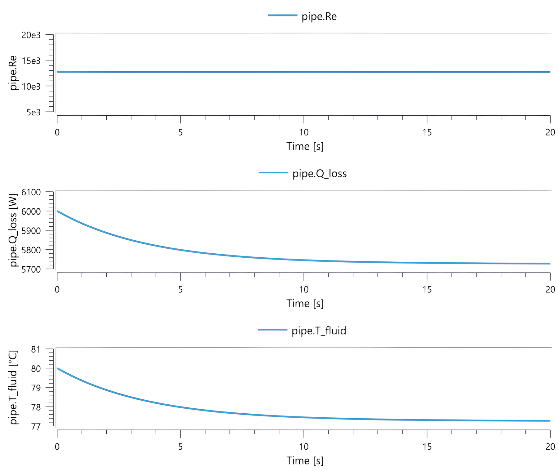
PipeSystem over 20 s: Re constant at ~12,700, Qloss decreasing as Tfluid decays exponentially toward steady state.
The matching result plot for the model above. Three quantities tell a coherent story: Reynolds number stays in the turbulent regime throughout, the wall heat flux falls as the fluid cools, and the fluid temperature decays smoothly toward the ambient-influenced steady state. A clean separation of timescales — and exactly the kind of multi-variable readout System Modeler's Simulation Center produces by default.
9. Data integration — wind turbine
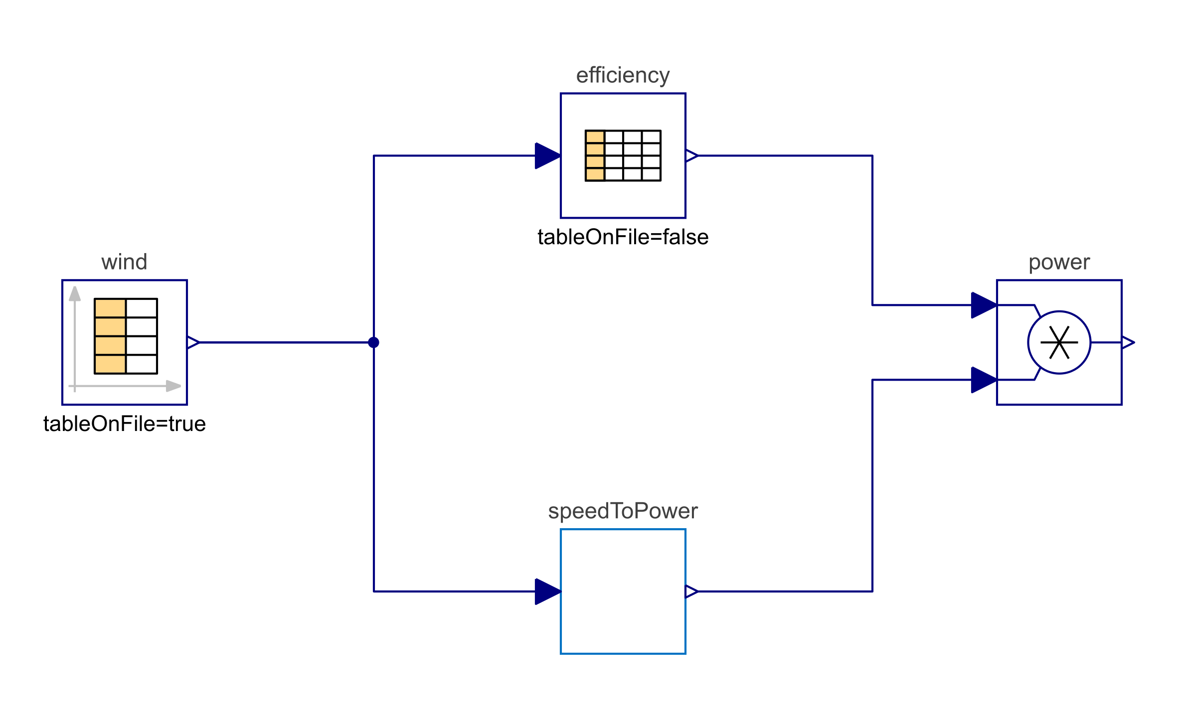
Full data chain: a CombiTimeTable feeds wind speed to both an efficiency lookup and a power block; their outputs multiply to give actual power.
Engineers often ask: "what do I do when I don't have equations?" Many real components — heat pumps, compressors, rotor blades — are characterized by manufacturer curves or measurement data, not closed-form physics. Modelica's CombiTable family lets you connect tabular data directly into the same diagram as your equation-based components, and the solver treats them consistently with everything else. Here, time-series wind speed flows into an efficiency curve and a cubic-power model, and the product is the turbine's actual output.
10. Inside the compiler — the symbolic preprocessing pipeline
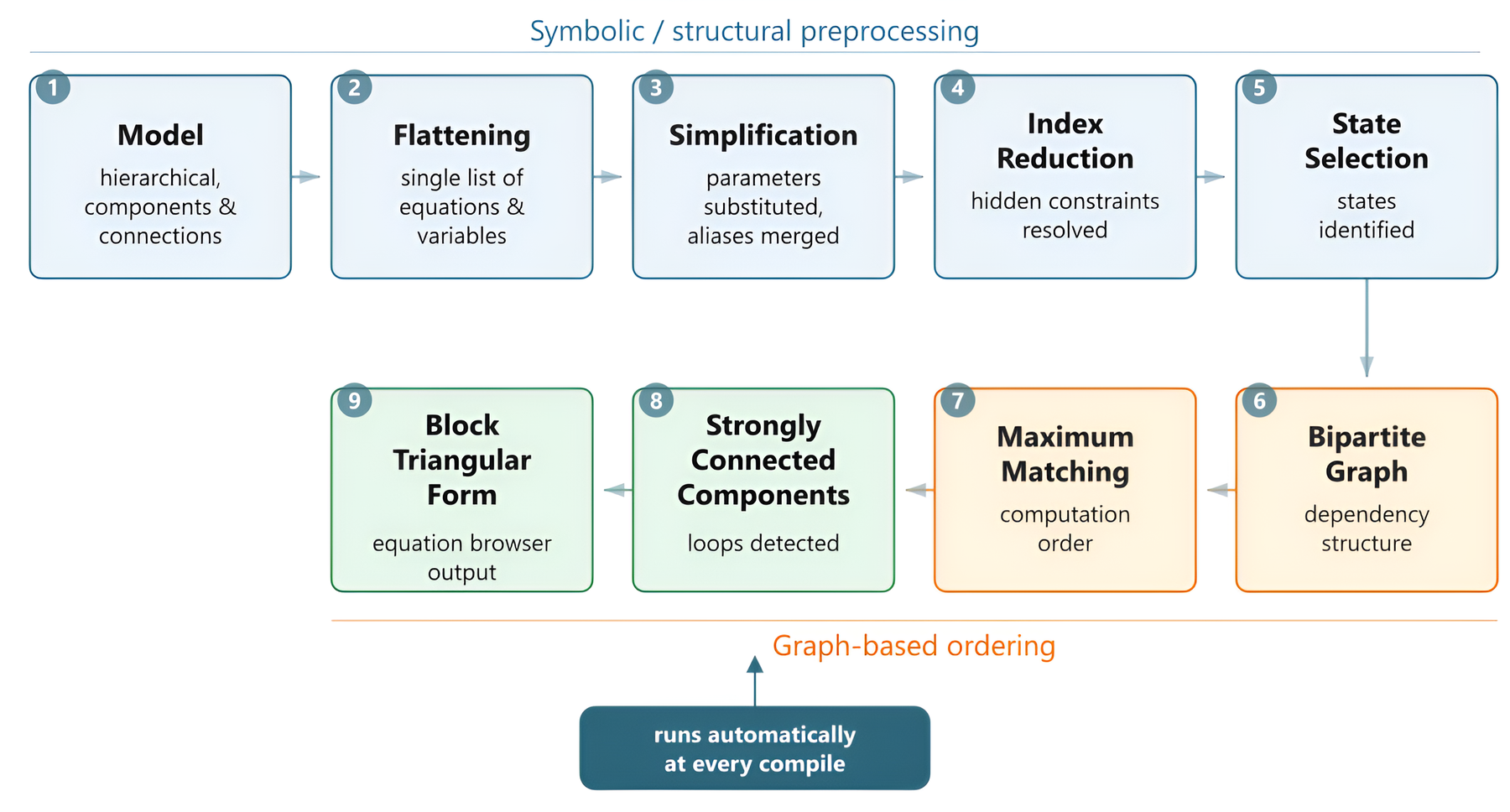
The symbolic preprocessing pipeline: from hierarchical model to block triangular form, runs automatically at every compile.
When a Modelica tool compiles a model it isn't just translating code — it's performing a sequence of symbolic transformations: flattening the hierarchy, simplifying, reducing differentiation index, selecting state variables, building a bipartite dependency graph, finding a maximum matching, breaking strongly connected components, and emitting block-triangular code the numerical solver can step through. The user never sees this; the user just sees a model that runs.
11. The bipartite graph behind every Modelica model
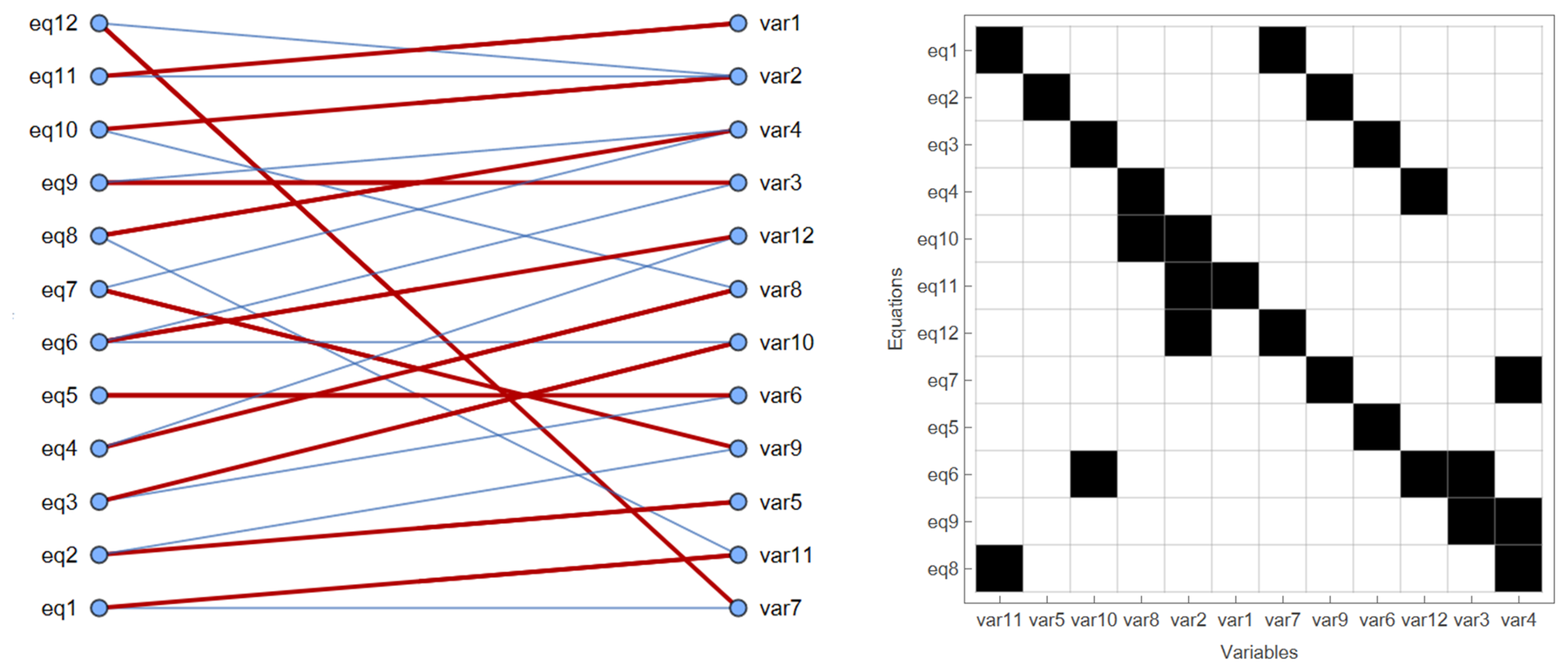
Maximum matching assigns each equation to the one variable it solves; the thick edges define the computation direction.
This is the moment a Modelica model becomes solvable. Equations and variables form a bipartite graph; an edge means "this variable appears in this equation." A maximum matching pairs each equation with the unique variable it will be used to compute — turning an undirected web of relations into a directed computation order. The same picture, shown as an incidence matrix on the right, is how a sparse linear-algebra package would see it. (The kind of structure a Wolfram Language audience tends to enjoy.)
12. FMI — Modelica's tool-interoperability story
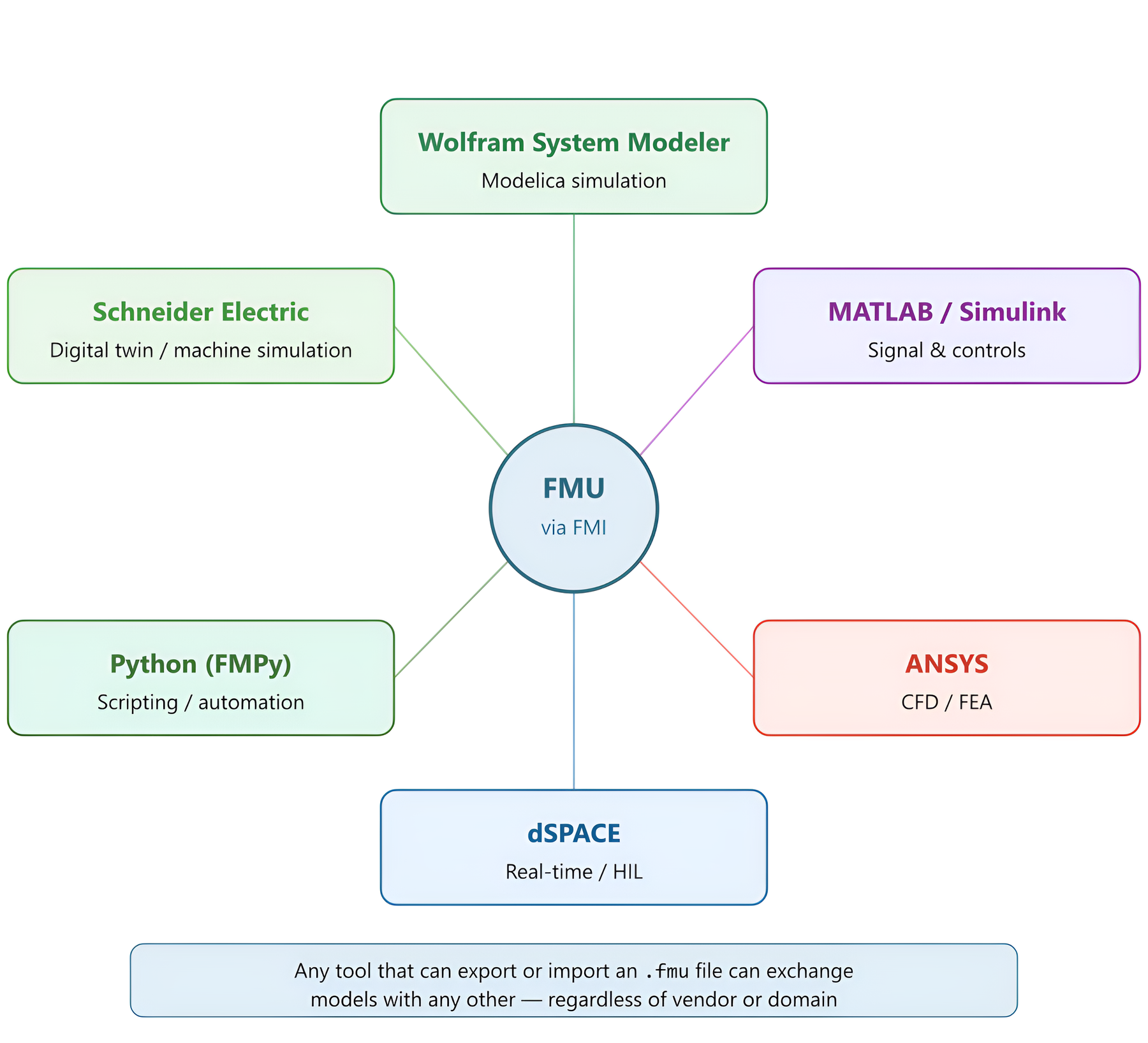
FMI as a universal connector: an FMU exported from any tool can be imported by any other FMI-compliant tool.
Once a model is built, the Functional Mock-up Interface (FMI) lets it cross tool boundaries. A Wolfram System Modeler component can be exported as an FMU, dropped into a Simulink controller study, embedded in a Python automation script, or run on dSPACE real-time hardware-in-the-loop. The simulation asset outlives any single tool — a real concern for long-lived models in aerospace, automotive, and energy.
13. The Modelica landscape — what the book covers
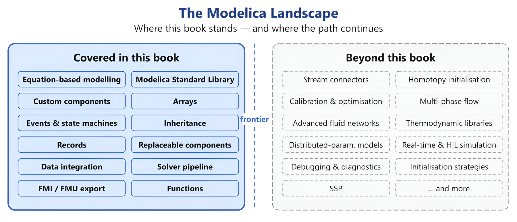
What this book covered vs. what lies beyond: a map of where you stand and where the path continues.
A reader's-eye view of the book's scope. On the left, the topics the book takes the reader through to fluency: equation-based modelling, the standard library, custom components, events and state machines, records, arrays, inheritance, replaceable components, data integration, FMU export, the solver pipeline, and functions. On the right, the topics that lie beyond — stream connectors, homotopy initialisation, multi-phase flow, real-time/HIL — pointing the reader to where to go next.
14. Application gallery — a building chiller
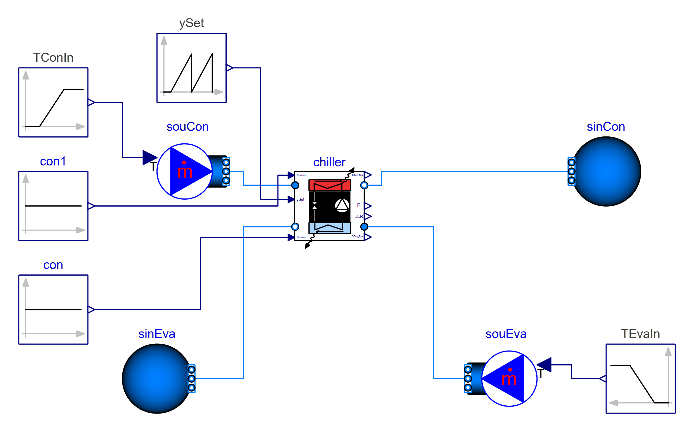
Chiller model from the Buildings library: condenser and evaporator loops connected through the chiller, with control inputs and fluid boundary conditions.
Modelica's reach into building energy simulation is substantial. The Buildings library (developed at LBNL) provides hundreds of validated HVAC components — chillers, heat pumps, fans, control sequences — that compose into whole-building models suitable for design and operational studies. This figure shows a single chiller with its condenser and evaporator loops; full plant models scale to thousands of components.
15. Application gallery — a DC motor drive
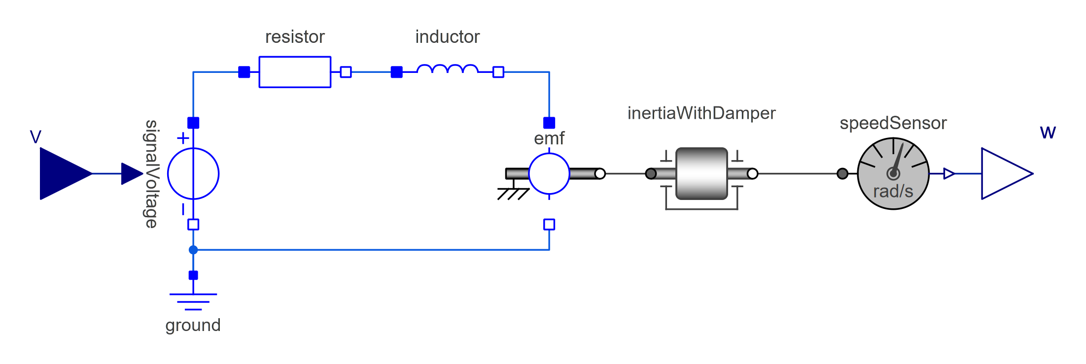
DC motor drive model: a voltage source drives current through the EMF, which converts electrical energy to rotational motion against a load.
The DC motor is the textbook example of an acausal multi-domain model — and it's also a real component that ships in countless products. One diagram crosses two physical domains: the electrical loop (resistor, inductor, EMF) and the rotational mechanical loop (inertia, damper, speed sensor). The energy conversion at the EMF couples the two automatically through the connector equations. Set the input voltage profile and the speed comes out; reverse the boundary conditions and the same model behaves as a generator.


