In the famous book "Understanding Molecular Simulation: From Algorithms to Applications" by D. Frenkel and B. Smit, there is a case study to use Monte Carlo (MC) molecular simulation computing the phase diagram of Lennard-Jones fluid. The results shall be compared with data compiled by Johnson et al [1]. The source code provided with the book, however, can only be compiled under Fortran 77 with Linux command line. With Mathematica at hand, it is tempting to rewrite these code and offer myself with a more intuitive and flexible viewpoint to the problem.
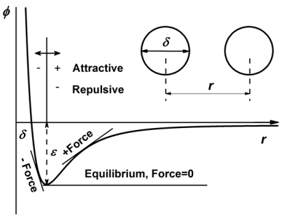
The LJ potential is given by
$$\phi(r)=4\epsilon \left[\left(\frac{\sigma}{r}\right)^{12}-\left(\frac{\sigma}{r}\right)^6\right]$$
where $\phi$, $\epsilon$, $\sigma$ and $r$ are illustrated below.
First, there should be a box of lattice particles.
 latticeDisplace[boxSize_?NumberQ,numParticle_Integer]:=
    Block[{delta=boxSize/Ceiling@(numParticle^((1/3))),flag=1,position=ConstantArray[{0,0,0},numParticle]},
        Do[
           Do[
             Do[{If[flag<=numParticle,position[[flag]]={xComponent,yComponent,zComponent}],flag++},{zComponent,delta/2.,boxSize,delta}],
           {yComponent,delta/2.,boxSize,delta}],
        {xComponent,delta/2.,boxSize,delta}];
        Return[position];
    ]";
At the cut-off distance $r_c$, one can choose to do either truncation $\phi(r)=0$ for $r>r_c$ or shift $\phi(r)=\phi(r)-\phi(r_c)$ for $r < r_c$. The virial potential is calculated as
$$Vir(r) = force \times r = -r\frac{d\phi(r)}{dr}=48\epsilon \left[\left(\frac{\sigma}{r}\right)^{12}-0.5\left(\frac{\sigma}{r}\right)^6\right]$$
ener[cutoffSquare_?NumberQ, distanceSquare_?NumberQ, \[Sigma]Square_?NumberQ, \[Epsilon]_?NumberQ, shift_]:=
    Block[{energy, vir},
    If[distanceSquare<cutoffSquare,
    {energy=4.\[Epsilon]((\[Sigma]Square/distanceSquare)^6-(\[Sigma]Square/distanceSquare)^3)-If[shift,4.\[Epsilon]((\[Sigma]Square/cutoffSquare)^6-(\[Sigma]Square/cutoffSquare)^3),0],vir=48.\[Epsilon]((\[Sigma]Square/distanceSquare)^6-.5(\[Sigma]Square/distanceSquare)^3)},
    {energy=0,vir=0}];
    Return[{energy, vir}]
   ];
Then, introduce periodic boundary condition if the distance between any two particles is larger than half box size.
potential[posi_, particleID_Integer, startParticle_Integer:1, {boxSize_?NumberQ, cutoffSquare_?NumberQ, \[Sigma]Square_, \[Epsilon]_, shift_}]:=
    Block[{length=Range[startParticle, Length@posi],distanceSquare,(*{energy,vir}={0,0}*)energy=0, vir=0},
        Do[
           If[part!=particleID,
             {distanceSquare=
              If[Norm[posi[[particleID]]-posi[[part]]]^2>boxSize^2/4,
              Norm[posi[[particleID]]-posi[[part]]/.dis_/;Abs@dis>boxSize/2->boxSize-Abs@dis]^2(*(boxSize-Norm[posi[[particleNum]]-posi[[part]]])^2*),
              Norm[posi[[particleID]]-posi[[part]]]^2],
              {energy,vir}+=ener[cutoffSquare, distanceSquare,\[Sigma]Square, \[Epsilon], shift]}],
        {part, startParticle, Length@posi}];
    Return[{energy, vir}]
  ];
The pressure tail at cut-off distance is
$$P_{tail}=\frac{16}{3} \pi \rho ^2 \sigma ^3 \epsilon \left[\frac{2}{3} \left(\frac{\sigma }{r_c}\right)^9-\left(\frac{\sigma }{r_c}\right)^3\right]$$
tailPressure[{cutoffSquare_?NumberQ, \[Sigma]Square_, \[Epsilon]_}, \[Rho]_?NumberQ]:=
Block[{\[Sigma]=Sqrt@\[Sigma]Square, rc=Sqrt@cutoffSquare, correctPressure},
correctPressure=16/3*\[Pi]*\[Epsilon]*\[Rho]^2*\[Sigma]^3 (2/3 (\[Sigma]/rc)^9-(\[Sigma]/rc)^3);
Return[correctPressure]
]
Similarly, the energy tail at cut-off is
$$\phi_{tail}=\frac{8}{3} \pi \rho \sigma ^3 \epsilon \left[\frac{1}{3} \left(\frac{\sigma }{r_c}\right)^9-\left(\frac{\sigma }{r_c}\right)^3\right]$$
tailEnergy[{cutoffSquare_?NumberQ, \[Sigma]Square_, \[Epsilon]_}, \[Rho]_?NumberQ]:=
Block[{\[Sigma]=Sqrt@\[Sigma]Square, rc=Sqrt@cutoffSquare, correctEnergy},
correctEnergy=8/3*\[Pi]*\[Epsilon]*\[Rho]*\[Sigma]^3 (1/3 (\[Sigma]/rc)^9-(\[Sigma]/rc)^3);
Return[correctEnergy]
]
With potential[] and tailEnergy[], the total energy $\Phi$ of all particles inside the ensemble can be calculated.
totalEnergy[posi_,tailCor_,{boxSize_?NumberQ, cutoffSquare_?NumberQ, \[Sigma]Square_, \[Epsilon]_, shift_}]:=
Block[{length=Length@posi, totalEnergy=0, totalVir=0, \[Rho]},

    Do[
       {totalEnergy, totalVir}+=potential[posi,particle,particle,{boxSize, cutoffSquare, \[Sigma]Square, \[Epsilon], shift}]

    ,{particle, 1, length}];

    If[tailCor,
       {\[Rho]=length/boxSize^3,
       totalEnergy+=length*tailEnergy[{cutoffSquare,\[Sigma]Square, \[Epsilon]},\[Rho]]}
    ];

    Return[{totalEnergy, totalVir}]
]
For monatomic particles, there is only translational moves to be considered. Otherwise orientational moves need to be taken into account (Rigid/Nonrigid, Linear/Nonlinear). For Monte Carlo algorithm:
- Randomly select one particle from the ensemble and calculate the system potential $\Phi_i$.
- Have the particle a random displacement $r`=r+\Delta$, and calculate the new system potential $\Phi_n$.
- Accept the trial move in last step with probability $exp[-(\Phi_n-\Phi_i)/kT]$
Code:
mcTranslate[posi_ , dr_, \[Beta]_,{boxSize_?NumberQ, cutoffSquare_?NumberQ, \[Sigma]Square_, \[Epsilon]_, shift_}]:=
    Block[
       {flag=RandomInteger[{1, Length@posi}], oldConf, oldPotential=0, oldVir=0, newPotential=0, newVir=0, config = posi, numAcc=0, potentialDiff=0, virDiff=0},
         {oldPotential, oldVir}=potential[config, flag, 1, {boxSize, cutoffSquare, \[Sigma]Square, \[Epsilon], shift}];
         oldConf = config[[flag]];
         config[[flag]] += dr*RandomReal[{-.5, .5},{3}];
         config[[flag]]=config[[flag]]/.dis_/;dis>boxSize->dis-boxSize;
         config[[flag]]=config[[flag]]/.dis_/;dis<0->boxSize+dis;
         {newPotential, newVir}=potential[config, flag, 1, {boxSize, cutoffSquare, \[Sigma]Square, \[Epsilon], shift}];
       If[
         RandomReal[]<Exp[-\[Beta](newPotential-oldPotential)],
         {++numAcc,potentialDiff+=(newPotential-oldPotential), virDiff+=(newVir-oldVir)},
         {config[[flag]]=oldConf}
       ];
       Return[{numAcc, potentialDiff, virDiff, config}];
]


monteCarlo[posi_, attemp_, stepSpace_, temp_, {boxSize_?NumberQ, cutoffSquare_?NumberQ, \[Sigma]Square_, \[Epsilon]_, shift_}]:=
Block[{acceptNum=0, energyDif=0, virDif=0, configuration=posi, numAccept=0, difEnergy=0, difVir=0},
    Nest[
    (
       {acceptNum, energyDif, virDif, configuration}=mcTranslate[#, stepSpace, 1/temp, {boxSize, cutoffSquare, \[Sigma]Square, \[Epsilon], shift}];
       numAccept+=acceptNum;
       difEnergy+=energyDif;
       difVir+=virDif;
       configuration
       (*Print[{energy, vir, configuration}];*)
    )&,
    configuration,
    attemp
    ];

Return[{numAccept/attemp//N, difEnergy, difVir, configuration}]
]
Another trick is to adjust the trial step $\Delta$ so that the accept ratio is around 0.5 (or any value between 0 and 1). If it's too large, more trials would be rejected, while too small value leads to longer computational time reaching equilibrium. Also, any new $\Delta$ should be compared with box size to comply with periodic boundary condition.
adjustStep[frac_, stepSpace_, targetFrac_:0.5, boxSize_]:=
Block[{stepOrigin=stepSpace, stepNew},
stepNew=stepSpace*frac/targetFrac;
If[stepNew/stepOrigin>1.5,stepNew=1.5stepOrigin];
If[stepNew/stepOrigin<.5,stepNew=.5stepOrigin];
If[stepNew>.5boxSize,stepNew=.5boxSize];

Return[stepNew];
]
Finally the thermodynamic properties can be calculated including specific energy and pressure.
propertyThermo[posi_, ener_, vir_, temperature_, {boxSize_, cutoffSquare_?NumberQ, \[Sigma]Square_, \[Epsilon]_}, tailCor_:True]:=
Block[{averageEnergy=ener/Length@posi, volume=boxSize^3, density=Length@posi/boxSize^3, pressure},
(*Print[boxSize,volume];*)
pressure=Length@posi/volume*temperature+vir/(3*volume);
(*Print[pressure,volume];*)
If[tailCor,pressure+=tailPressure[{cutoffSquare, \[Sigma]Square, \[Epsilon]}, \[Rho]]];
Return[{averageEnergy, pressure}];
]
Intuitive animation enables a directive observation to the ensemble energy profile, which makes it possible to determine whether the simulation cycle and trial numbers are sufficient for the system to reach equilibrium.

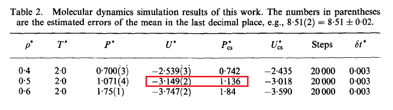
Parameters for the test run is $\rho=0.5$, $T=2$, particle number is 200. MC runs 40 cycles, in each of which there are 1,000 trial moves. LJ potential at cut-off is truncated, and pressure tail is corrected. The results is $P=1.12461$ and average internal energy $-3.1517$. This is an excellent agreement with data from Johnson et al [1], at their Table 2.
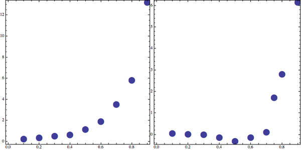
D. Frenkel et al also presented the LJ equation of state isotherm at $T=2.0$ and $T=0.9$. A comparison between their results and this work is given below.
D. Frenkel et al:
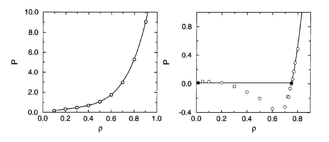
This work:
[1] J. Johnson, J. Zollweg, K. Gubbins, The Lennard-Jones equation of state revisited, Mol. Phys. 78 (1993) 591618.
The code is tested under MMA 9.0.


