Dear Community,
I have been going over the documentation for the use of ParametricNDSolve[], and was wondering about the meaning of one of the basic examples provided in the documentation.
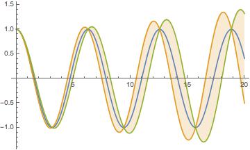
In the example, we are trying to show the sensitivity of a solution provided by ParametricNDSolve[], of a differential equation with two-parameter inputs. The equation is:
sol = ParametricNDSolve[{y''[t] + a y[t] == 0, y[0] == b, y'[0] == 0},
   y, {t, 0, 20}, {a, b}];
If looking at the sensitivity of variable a with respect to time t, the code is:
Plot[Evaluate[(y[1, 1][t] + {0, .1, -.1} D[y[a, 1], a][t] /.
     a -> 1) /. sol], {t, 0, 20}, Filling -> {2 -> {3}}]
Yielding the following plot:
The same is done for the analysis of b (which I left out, as I suspect the above plot will be enough for a helpful soul to dumb it down to my level of understanding :-) ).
My question is, what exactly is shown? Lets for instance say that y(t) is the population of ticks within a defined area. The population is dependent on the temperature (say, variable a), and the humidity (variable b). Then:
y[1,1][t]
would correspond to evaluating a base case scenario where a=b=1. To this expression we then add:
{0, .1, -.1} D[y[a, 1], a][t] /. a -> 1
When multiplying the differential by 0, we get the base case, but is correctly understood that {.1,-.1} multiplied with the differential, gives the base case value, with the effect of a 10% change in a at time t, by finding the rate of change of y(t), with respect to a, and then evaluating the rate (or slope) at a=1.
But even so, does this tell me that the effect of a 10% change of a would be more significant at later times, rather than at the very beginning? or am I way off?
Sorry for the long post!
Best Regards


